In continual learning problems, it is often necessary to overwrite components of a neural network’s learned representation in response to changes in the data stream; however, neural networks often exhibit primacy bias, whereby early training data hinders the network’s ability to generalize on later tasks. While feature-learning dynamics of nonstationary learning problems are not well studied, the emergence of feature-learning dynamics is known to drive the phenomenon of grokking, wherein neural networks initially memorize their training data and only later exhibit perfect generalization. This work conjectures that the same feature-learning dynamics which facilitate generalization in grokking also underlie the ability to overwrite previous learned features as well, and methods which accelerate grokking by facilitating feature-learning dynamics are promising candidates for addressing primacy bias in non-stationary learning problems. We then propose a straightforward method to induce feature-learning dynamics as needed throughout training by increasing the effective learning rate, i.e. the ratio between parameter and update norms. We show that this approach both facilitates feature-learning and improves generalization in a variety of settings, including grokking, warm-starting neural network training, and reinforcement learning tasks.
継続学習問題では、データストリームの変化に応じてニューラルネットワークの学習済み表現のコンポーネントを上書きする必要があることがよくあります。しかし、ニューラルネットワークはプライマシーバイアスを示すことが多く、初期のトレーニングデータがネットワークの後のタスクにおける一般化能力を阻害します。非定常学習問題の特徴学習ダイナミクスは十分に研究されていませんが、特徴学習ダイナミクスの出現がグロッキング現象を促進することが知られています。グロッキング現象では、ニューラルネットワークは最初にトレーニングデータを記憶し、後になって初めて完全な一般化を示します。本研究では、グロッキングにおける一般化を促進するのと同じ特徴学習ダイナミクスが、以前に学習した特徴を上書きする能力の基盤にもなっていると推測しており、特徴学習ダイナミクスを促進することでグロッキングを加速する手法は、非定常学習問題におけるプライマシーバイアスに対処するための有望な候補です。次に、実効学習率、すなわちパラメータと更新ノルムの比率を増加させることで、訓練全体を通して必要に応じて特徴学習ダイナミクスを誘導する簡便な手法を提案する。この手法は、グロッキング、ウォームスタートによるニューラルネットワーク訓練、強化学習タスクなど、様々な設定において、特徴学習を促進し、汎化を向上させることを示す。
Non-stationarity is ubiquitous in real-world applications of AI systems: datasets may grow over time, correlations may appear and then disappear as trends evolve, and AI systems themselves may take an active role in the generation of their own training data. However, neural network training algorithms typically assume a fixed data distribution, and successfully training a neural network in non-stationary conditions requires avoiding a variety of potential failure modes, including loss of plasticity (Lyle et al., 2021; Dohare et al., 2021; Abbas et al., 2023), where the network becomes less able to reduce its training loss over time, and primacy bias (Ash & Adams, 2020; Nikishin et al., 2022), where early data impede the network’s ability generalize well on later tasks1. While many prior works have analyzed the learning dynamics that lead to loss of plasticity, comparatively less attention has been paid to the learning dynamics underlying degraded generalization ability. Current approaches to address the problem include perturbation or complete re-initialization of the network parameters (Ash & Adams, 2020; Schwarzer et al., 2023; Lee et al., 2023) or regularization in some form towards the initialization distribution (Lyle et al., 2021; Kumar et al., 2023) or initial conditions (Lewandowski et al., 2025), a solution which, while effective, can transiently reduce performance and does not provide insight into why the network fails to generalize in the first place.
非定常性は、AI システムの実際のアプリケーションに遍在します。データセットは時間の経過とともに増加し、相関関係はトレンドの進化に伴って現れては消え、AI システム自体が独自のトレーニングデータの生成に積極的な役割を果たす場合があります。しかし、ニューラルネットワークのトレーニングアルゴリズムは通常、固定のデータ分布を前提としており、非定常条件下でニューラルネットワークを正常にトレーニングするには、可塑性の喪失 (Lyle et al., 2021; Dohare et al., 2021; Abbas et al., 2023) やプライマシーバイアス (Ash & Adams, 2020; Nikishin et al., 2022) など、さまざまな潜在的な障害モードを回避する必要があります。可塑性の喪失は、ネットワークが時間の経過とともにトレーニング損失を削減する能力が低下することを意味し、プライマシーバイアス (Ash & Adams, 2020; Nikishin et al., 2022) は、初期のデータがネットワークの後のタスクでの一般化能力を阻害することを意味します1。可塑性の喪失につながる学習ダイナミクスは多くの先行研究で分析されてきたものの、汎化能力の低下の根底にある学習ダイナミクスについては比較的注目されてきませんでした。この問題に対処するための現在のアプローチとしては、ネットワークパラメータの摂動または完全な再初期化(Ash & Adams, 2020; Schwarzer et al., 2023; Lee et al., 2023)、あるいは初期化分布(Lyle et al., 2021; Kumar et al., 2023)もしくは初期条件(Lewandowski et al., 2025)に向けた何らかの形の正則化などが挙げられますが、これらの解決策は効果的ではあるものの、一時的にパフォーマンスを低下させる可能性があり、そもそもネットワークが汎化に失敗する理由についての洞察は得られません。
In this paper, we will propose a framework for understanding and mitigating this degradation in generalization performance which connects three previously disparate phenomena: primacy bias, grokking, and feature-earning dynamics.
本稿では、プライマシーバイアス(初頭バイアス)、グロッキング、特徴獲得ダイナミクスという、これまでは別個の現象として認識されていた 3 つの現象を結び付け、一般化パフォーマンスの低下を理解し、軽減するためのフレームワークを提案します。
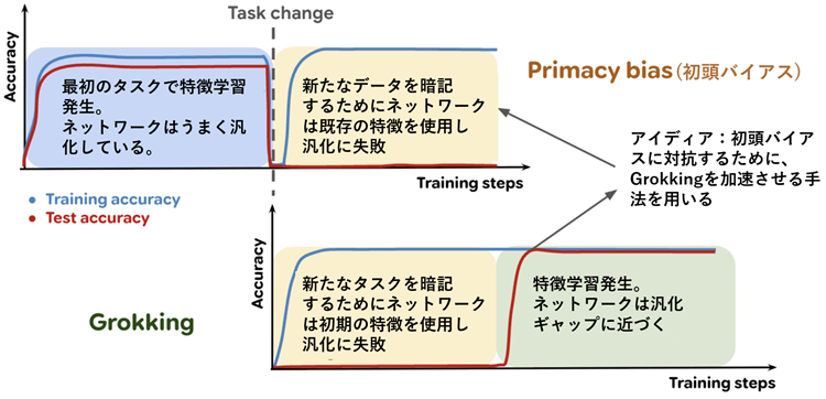
Concretely, we investigate the hypothesis that the same fundamental process by which a network replaces randomly initialized memorizing features with generalizing ones during grokking can be leveraged in continual learning problems to overwrite previously-learned features with new ones. Thus, a method which accelerates grokking (e.g., in modular arithmetic problems where this phenomenon is typically examined) will be expected to also mitigate primacy bias in non-stationary learning problems. We visualize this analogy in Figure 1, which illustrates how the memorization and (possible) feature-learning phase of grokking can be mapped onto the continual learning setting. We go on to make three primary contributions.
具体的には、ネットワークがグロッキング(grokking)時にランダムに初期化された記憶特徴を一般化特徴に置き換えるという同じ基本プロセスが、継続学習問題において、既に学習した特徴を新しい特徴で上書きするために利用できるという仮説を検証します。したがって、グロッキングを加速する手法(例えば、この現象が典型的に検討されるモジュラー算術問題)は、非定常学習問題におけるプライマシーバイアスを軽減することも期待されます。このアナロジーを図1に示します。これは、グロッキングにおける記憶段階と(場合によっては)特徴学習段階が、継続学習環境にどのようにマッピングできるかを示しています。私たちはさらに、3つの主要な貢献を行います。
Figure 1: Both primacy bias (top row) and grokking (bottom row) exhibit a period where the network exhibits poor generalization due to an absence of feature-learning (yellow). In primacy bias, this is due to unsuitable learned features from the initial training phase (blue). In grokking, the network eventually recovers feature-learning dynamics (green) and generalizes.
図1:プライマシーバイアス(上段)とグロッキング(下段)はどちらも、特徴学習の欠如(黄色)によりネットワークの汎化能力が低下する期間を示しています。プライマシーバイアスでは、これは初期学習段階で学習した不適切な特徴(青)が原因です。グロッキングでは、ネットワークは最終的に特徴学習のダイナミクス(緑)を回復し、汎化能力を発揮します。
First, based on the above hypothesis, we develop a unifying framework for understanding grokking and primacy bias as the emergence (or lack thereof) of feature-learning dynamics (Section 3).
まず、上記の仮説に基づいて、グロッキングとプライマシーバイアスを特徴学習ダイナミクスの出現(またはその欠如)として理解するための統一的な枠組みを開発します(セクション3)。
Second, to translate the above framework into an algorithm, we propose a simple modification to the Normalize and Project method of Lyle et al. (2024a), which addresses the loss of plasticity problem by avoiding the excessive decay of the effective learning rate (ELR) – a scale-invariant interpretation of the learning rate which takes into account the magnitude of the parameter norms, as defined in Section 2 – during the training process. We show that increasing the effective learning rate after it has decayed, a process which we will refer to as ELR re-warming, induces feature-learning dynamics, and propose a simple method (Algorithm 1 in Section 3.1) that allows the ELR to be re-warmed periodically throughout training, recovering feature-learning dynamics outside of the initial learning period.
次に、上記のフレームワークをアルゴリズムに変換するために、Lyle ら (2024a) の正規化および投影法に単純な修正を加えることを提案する。この修正は、トレーニングプロセス中の有効学習率 (ELR) の過度な減衰を回避することで可塑性喪失問題に対処するものである。ELR とは、第 2 節で定義したように、パラメータノルムの大きさを考慮した学習率のスケール不変な解釈である。有効学習率が減衰した後にそれを増加させること (ELR 再加温と呼ぶ) により、特徴学習ダイナミクスが誘発されることを示し、トレーニング全体を通して ELR を定期的に再加温して、初期学習期間外で特徴学習ダイナミクスを回復できるようにする単純な方法 (第 3.1 節のアルゴリズム 1) を提案する。
Finally, we successfully apply ELR re-warming to improve generalization on both stationary and non-stationary domains. We consider three primary applications: grokking (Section 4), where the dataset is fixed and generalization requires over-writing the features provided by the random initialization; warm-starting image classification (Section 5), where the network is trained on a dataset which grows over time as more data is added; and finally reinforcement learning (Section 6), where not only the input distribution, but also the relationship between input and prediction target itself, is in flux. The success of our method in these different domains demonstrates that ELR rewarming does not depend on any special structure of the features which might arise during initialization or learning features for a given task.
最後に、ELRリウォーミングを適用することで、定常領域と非定常領域の両方で一般化を向上させることに成功しました。主な応用分野は3つあります。グロッキング(セクション4)ではデータセットが固定されており、一般化にはランダム初期化によって提供された特徴の上書きが必要です。ウォームスタート画像分類(セクション5)では、ネットワークはデータセットに追加されるにつれて時間の経過とともに成長します。最後に、強化学習(セクション6)では、入力分布だけでなく、入力と予測対象自体の関係も変化します。これらの異なる領域における本手法の成功は、ELRリウォーミングが、特定のタスクの初期化または特徴学習中に生じる可能性のある特徴の特別な構造に依存しないことを示しています。
Taken in the context of prior work, this paper presents a radically simplified model for primacy bias and its mitigation which is corroborated empirically in a diverse set of domains. Our analysis also reveals a trade-off analogous to that between stability and plasticity: increasing the effective learning rate allows the network shake off the influence of irrelevant early training data, but this increase must be transient to allow the optimization process to make fine-grained modifications to the network outputs necessary for optimal performance. Our findings thus present a promising springboard for further work developing the ELR as a means of navigating the landscape of plasticity-stability tradeoffs in continual learning.
本論文は、先行研究を踏まえ、プライマシーバイアスとその緩和策について、根本的に単純化されたモデルを提示する。このモデルは、多様な領域において実証的に裏付けられている。また、我々の分析は、安定性と可塑性の間に見られるトレードオフに類似するトレードオフも明らかにしている。すなわち、実効学習率の増加は、ネットワークが初期の無関係な学習データの影響を振り払うことを可能にする。しかし、最適化プロセスが最適なパフォーマンスを得るために必要なネットワーク出力へのきめ細かな修正を行うためには、この増加は一時的なものでなければならない。したがって、我々の発見は、継続学習における可塑性と安定性のトレードオフという難題を乗り越える手段としてのELRの開発に向けた、今後の研究にとって有望な足がかりとなる。
This work provides a unifying perspective on feature learning in neural networks, connecting the disparate phenomena of plasticity loss, the failure to adapt features to new learning signals, and grokking, the acquisition of feature-learning
dynamics after interpolation has been achieved. This section provides background on each of these topics and introduces
the concept of an effective learning rate, which will play a critical role in our proposed method.
本研究は、ニューラルネットワークにおける特徴学習に関する統一的な視点を提供し、可塑性喪失(特徴が新しい学習信号に適応できないこと)とグロッキング(補間が達成された後に特徴学習ダイナミクスを獲得すること)という異なる現象を結び付けています。本節では、これらの各トピックの背景を説明し、提案手法において重要な役割を果たす有効学習率の概念を紹介します。
Training a neural network on a sequence of tasks has been demonstrated to interfere with its ability to adapt to new
information, a phenomenon which we will refer to as loss of plasticity (Dohare et al., 2021; Lyle et al., 2021; Nikishin et al., 2022; Dohare et al., 2024). Loss of plasticity has been demonstrated to impair performance in a number of RL tasks (Igl et al., 2021; Lyle et al., 2023; Nikishin et al., 2023), as well as in non-stationary supervised learning problems (Ash & Adams, 2020; Berariu et al., 2021). Plasticity loss can take the form of an inability to minimize the training objective in response to changes in the data distribution, occurring in sequential learning of unrelated tasks (Lyle et al., 2021), or an inability to generalize to new, unseen inputs, as occurs in warm-starting (Lee et al., 2024). A variety of approaches to mitigate plasticity loss have been proposed, such as regularization towards the initial parameters (Kumar et al., 2023), the use of normalization layers (Lyle et al., 2024a), weight clipping (Elsayed et al., 2024), perturbation or partial resetting of the network parameters (Dohare et al., 2023), and spectral regularization (Lewandowski et al., 2025). Loss of plasticity has been further tied both to reductions in the network’s effective step size as a result of parameter norm growth (Lyle et al., 2024b) as well as changes in the network’s curvature (Lewandowski et al., 2023), quantities which have exhibited deep connections in stationary supervised learning settings via the catapult mechanism (Lewkowycz et al., 2020), implicit regularization (Barrett & Dherin, 2020), and
edge-of-stability dynamics (Cohen et al., 2021; Agarwala et al., 2022; Roulet et al., 2023). We will show in this work
that not only does avoiding excessive decay in the effective learning rate mitigate plasticity loss, but that re-warming it
to a sufficient value can recover many of the beneficial feature-learning conditions observed in the large-learning-rate
early-training regime by prior works.
ニューラルネットワークを一連のタスクで学習させると、新しい情報への適応能力が損なわれることが実証されており、この現象を可塑性喪失と呼びます(Dohare et al., 2021; Lyle et al., 2021; Nikishin et al., 2022; Dohare et al., 2024)。可塑性喪失は、多くの強化学習タスク(Igl et al., 2021; Lyle et al., 2023; Nikishin et al., 2023)だけでなく、非定常な教師あり学習問題(Ash & Adams, 2020; Berariu et al., 2021)においてもパフォーマンスを低下させることが実証されています。可塑性損失は、データ分布の変化に応じて学習目標を最小化できないという形で現れ、無関係なタスクの逐次学習で発生します(Lyle et al., 2021)。また、ウォームスタートで発生するような、新しい未知の入力への一般化ができないという形で現れます(Lee et al., 2024)。可塑性損失を軽減するための様々なアプローチが提案されており、初期パラメータへの正則化(Kumar et al., 2023)、正規化層の使用(Lyle et al., 2024a)、重みクリッピング(Elsayed et al., 2024)、ネットワークパラメータの摂動または部分的なリセット(Dohare et al., 2023)、スペクトル正則化(Lewandowski et al., 2025)などが挙げられます。可塑性の喪失は、パラメータノルムの成長(Lyle et al., 2024b)の結果としてのネットワークの有効ステップサイズの減少と、ネットワークの曲率の変化(Lewandowski et al., 2023)の両方にさらに関連付けられています。これらの量は、カタパルトメカニズム(Lewkowycz et al., 2020)、暗黙の正則化(Barrett & Dherin, 2020)、および安定端ダイナミクス(Cohen et al., 2021; Agarwala et al., 2022; Roulet et al., 2023)を介して定常教師あり学習設定で深いつながりを示しています。本研究では、実効学習率の過度の低下を避けることで可塑性の低下を軽減できるだけでなく、実効学習率を十分な値まで再調整することで、先行研究で観察された大きな学習率の初期訓練段階で得られた多くの有益な特徴学習条件を回復できることを示します。
Grokking comprises part of a broader body of work studying delayed generalization (Belkin et al., 2019; Heckel
& Yilmaz, 2021; Davies et al., 2023). While first prominently observed in small transformers trained on modular
arithmetic (Liu et al., 2022a), grokking has since been identified in a range of tasks, including parity-learning and
image classification variants (Bautiste et al., 2024; Liu et al., 2022b). Grokking has been theoretically characterized as
a phase transition from “lazy” to “rich” learning dynamics. In the initial lazy phase, the network fits the training data
without fundamentally changing its internal representations, akin to a linear model (Jacot et al., 2018; Yang, 2019). The
subsequent, much slower, rich-learning phase involves a significant reorganization of the network’s learned features
into a more structured, generalizing solution (Xu et al., 2024; Kumar et al., 2024; Lyu et al., 2024). Theoretical
analysis of this transition is complemented by empirical observations of the structured features learned in networks
which grok (Nanda et al., 2023; Liu et al., 2022a). In modular arithmetic tasks, for instance, progress metrics can
identify the emergence of these generalizing features prior to the uptick in test performance, sometimes tracking the
formation of partially-generalizing solutions along the way (Nanda et al., 2023; Varma et al., 2023).
Grokkingは、遅延一般化を研究する広範な研究の一部です(Belkin et al., 2019; Heckel & Yilmaz, 2021; Davies et al., 2023)。モジュラー演算で学習された小規模なTransformerにおいて初めて顕著に観察されましたが(Liu et al., 2022a)、その後、パリティ学習や画像分類のバリエーションを含むさまざまなタスクで確認されています(Bautiste et al., 2024; Liu et al., 2022b)。Grokkingは理論的には、「lazy」学習ダイナミクスから「rich」学習ダイナミクスへの相転移として特徴付けられています。初期のlazyフェーズでは、ネットワークは線形モデルと同様に、内部表現を根本的に変更することなく、学習データに適合します(Jacot et al., 2018; Yang, 2019)。その後の、はるかにゆっくりとしたリッチラーニング段階では、ネットワークが学習した特徴がより構造化された一般化解へと大幅に再編成されます (Xu et al., 2024; Kumar et al., 2024; Lyu et al., 2024)。この遷移の理論的分析は、ネットワークで学習された構造化された特徴が理解されるという実証的観察によって補完されます (Nanda et al., 2023; Liu et al., 2022a)。例えば、モジュラー算術タスクでは、進捗指標によって、テストパフォーマンスの向上に先立ってこれらの一般化特徴の出現を特定することができ、その過程で部分的に一般化解の形成を追跡できる場合もあります (Nanda et al., 2023; Varma et al., 2023)。
A variety of works have drawn empirical connections between the parameter norm and grokking, noting, for example,
that phase transitions in the model’s generalization performance accompany periods of instability in the network’s
optimization dynamics and rapid increases in the parameter norm (Thilak et al., 2022). While there is a widely
observed correlation between the parameter norm and grokking, the causal relationship between weight norm and
delayed generalization remains unclear. Whereas Liu et al. (2022b) characterize grokking as the convergence of the
parameter norm towards a “goldilocks zone” (Fort & Scherlis, 2019) which allows for generalization, Varma et al.
(2023) argue the converse: grokking occurs when the optimizer converges to an “efficient” circuit which generalizes
well, from which point weight decay can reduce the parameter norm without harming accuracy. This work bridges the
gap towards a causal understanding of the relationship by shedding light on the mechanisms by which the parameter
norm can influence the onset of grokking in Section 4, finding some truth in both perspectives.
様々な研究において、パラメータノルムとグロッキングの間には経験的な関連性が指摘されており、例えば、モデルの汎化性能における相転移は、ネットワークの最適化ダイナミクスの不安定期とパラメータノルムの急激な増加を伴うことが指摘されている (Thilak et al., 2022)。パラメータノルムとグロッキングの間には広く観察される相関関係がある一方で、重みノルムと遅延汎化との因果関係は依然として不明である。Liu et al. (2022b) はグロッキングを、パラメータノルムが汎化を可能にする「ゴルディロックスゾーン」(Fort & Scherlis, 2019) へと収束することと特徴づけているのに対し、Varma et al. (2023) は逆のことを主張している。すなわち、最適化器が「効率的な」回路に収束し、それがうまく一般化されると、グロッキングが発生し、その時点から重み減衰によってパラメータノルムを減少させても精度を損なうことはない。本研究は、第4節においてパラメータノルムがグロッキングの発生にどのように影響するかというメカニズムを明らかにし、両方の視点に一定の真実を見出すことで、関係性の因果的理解へのギャップを埋めている。
A crucial feature of our analysis in the sections that follow concerns the control of the effective learning rate,a quantity which has significant implications on learning dynamics (Arora et al., 2018; Li & Arora, 2020) in scale-invariant functions. While the learning rate has a large effect on how gradient-based optimizers perform in practice, this effect depends on the norm of the parameters and the gradients. The aim of the effective learning rate is to provide a metric independent of these quantities. Concretely, let \(f\) be a scale-invariant function for some \(α \neq 0\); that is, assume that \(f(θ)=f(αθ)\) for all \(θ\) in its domain. Then,
以降の節における分析の重要な特徴は、実効学習率の制御に関するものです。実効学習率は、スケール不変関数における学習ダイナミクス(Arora et al., 2018; Li & Arora, 2020)に重要な意味を持つ量です。学習率は勾配ベースの最適化器の実際のパフォーマンスに大きな影響を与えますが、この影響はパラメータと勾配のノルムに依存します。実効学習率の目的は、これらの量に依存しない指標を提供することです。具体的には、\(f\) をある \(α \neq 0\) に対するスケール不変関数とします。つまり、その定義域内のすべての \(θ\) に対して \(f(θ)=f(αθ)\) が成り立つと仮定します。すると、
\[
f(θ+η∇f(θ))=f(αθ+α^2η∇f(αθ)) \tag{1}
\]
and hence the effective learning rate \(\tilde{η}\) to replicate the learning dynamics on \(θ\) with unit-norm parameters \(\tilde{θ}\) is given by \(\tilde{η}(θ)=\frac{η}{|| θ||^2}\) for gradient descent (see e.g. Lyle et al. (2024a, Definition 1) for a derivation of this relationship) and \(\tilde{η}(θ)=\frac{η}{||θ||}\) in adaptive optimizers like RMSProp and Adam which approximate the update \(\frac{∇f(θ)}{||∇f(θ||)}\). Such arescaling is exact for scale-invariant functions, but even in networks which are only partially or approximately scale-invariant, such as those which include normalization layers, increased parameter norm is empirically associated with reduced sensitivity to gradient updates and loss of plasticity (Lyle et al., 2024b; Nikishin et al., 2022; Dohare et al., 2023). The relationship between parameter norm and effective learning rate is leveraged by Lyle et al. (2024a) in the Normalize and Project (NaP) algorithm, a method which aims to improve robustness to nonstationarity by maintaining tight control on the effective learning rate. NaP inserts normalization layers prior to each nonlinearity in the network and periodically projects the weights in each linear layer to the unit sphere (w.r.t. Frobenius norm \(||·||_F\) ), resulting in the two-step update for the matrix-valued parameters \(W^ℓ\) of each layer \(ℓ\), where \(u_t^ℓ\) denotes the optimizer update to \(W^ℓ\):
したがって、単位ノルムパラメータ \(\tilde{θ}\) を持つ \(θ\) 上の学習ダイナミクスを再現するための有効学習率 \(\tilde{η}\) は、勾配降下法では \(\tilde{η}(θ)=\frac{η}{|| θ||^2}\) で与えられ(この関係の導出については、例えば Lyle et al. (2024a、定義 1) を参照)、更新 \(\frac{∇f(θ)}{||∇f(θ||)}\) を近似する RMSProp や Adam などの適応型最適化装置では \(\tilde{η}(θ)=\frac{η}{||θ||}\) で与えられます。このような再スケーリングはスケール不変関数に対しては正確ですが、正規化層を含むネットワークなど、部分的にまたは近似的にスケール不変であるネットワークであっても、パラメータノルムの増加は経験的に勾配更新に対する感度の低下と可塑性の喪失と関連付けられています (Lyle et al., 2024b; Nikishin et al., 2022; Dohare et al., 2023)。パラメータノルムと実効学習率の関係は、Lyle et al. (2024a) によって正規化および投影 (NaP) アルゴリズムに利用されています。この手法は、実効学習率を厳密に制御することで非定常性に対する堅牢性を向上させることを目的としています。 NaP は、ネットワーク内の各非線形性の前に正規化レイヤーを挿入し、各線形レイヤーの重みを単位球面 (フロベニウス ノルム \(||·||_F\) に対して) に定期的に投影します。これにより、各レイヤー \(ℓ\) の行列値パラメーター \(W^ℓ\) の 2 段階更新が行われます。ここで、\(u_t^ℓ\) は \(W^ℓ\) への最適化更新を表します。
\[
\tilde{W}_t^ℓ ← W_{t-1}^ℓ+η_tu_t^ℓ, W_t^ℓ←\tilde{W}_t^ℓ\frac{||W_o^ℓ||_F}{||\tilde{W}_t^ℓ||} \tag{2}
\]
In some cases, it can be desirable to apply the projection step only every \(k\) updates either to reduce the computational overhead of the method or as an analytical means of interpolating between projection and regularization of the parameter norm. We will specify in later sections when this is the case, and default to projection every step. We will use this approach to ensure that the effective learning rate can be directly read off from the explicit learning rate schedule in later sections.
場合によっては、手法の計算オーバーヘッドを削減するため、あるいはパラメータノルムの投影と正則化の間の補間を解析的に行うため、\(k\) 回の更新ごとにのみ投影ステップを適用することが望ましい場合があります。この場合、ステップごとに投影をデフォルトで適用します。このアプローチは、後のセクションで明示的な学習率スケジュールから実効学習率を直接読み取ることができるようにするために使用します。
This section introduces the empirical and methodological tools which we will use to study the emergence of feature-learning in neural network training. Section 3.1 will present a set of empirical metrics which we will use to determine whether a network is meaningfully changing its learned representation, and Section 3.2 will propose a simple learning rate re-warming strategy to induce feature-learning dynamics on demand.
このセクションでは、ニューラルネットワークの学習における特徴学習の出現を研究するために用いる経験的および方法論的ツールを紹介します。3.1節では、ネットワークが学習した表現を意味のある形で変化させているかどうかを判断するために用いる一連の経験的指標を提示し、3.2節では、オンデマンドで特徴学習ダイナミクスを誘導するための、シンプルな学習率再加温戦略を提案します。
The dichotomy between kernel and feature-learning dynamics was first delineated in the study of infinite-width neural networks (Xiao et al., 2020; Yang, 2019), where for example Yang et al. (2022) define feature-learning as an \(Ω(1)\) change in the limiting feature covariance matrix of an intermediate layer of the network from its initial value as the
width increases. Under this definition, any finite-width network vacuously perform some amount of feature learning. What matters in practice, however, is the magnitude of the change undergone by the features, a quantity whose characterization admits a number of reasonable metrics. One such metric, inspired by the definition of Yang et al. (2022), is the change in the normalized feature covariance matrix at a given layer after some interval \(T\) . In particular, letting \(f^ℓ\) denote the output of layer \(ℓ\) and \(X\) denote some set of \(n\) training datapoints, with \(f^ℓ(X)∈\mathbb{R}^{n×d}\) denoting the matrix obtained by stacking the outputs for each datapoint, we define
カーネル学習ダイナミクスと特徴学習ダイナミクスの二分法は、無限幅ニューラルネットワークの研究で初めて明確に示された (Xiao et al., 2020; Yang, 2019)。例えば、Yang et al. (2022) は、特徴学習を、ネットワークの中間層の極限特徴共分散行列が、幅が増加するにつれて初期値から \(Ω(1)\) 変化するものとして定義している。この定義によれば、有限幅のネットワークは、空虚にいくらかの特徴学習を実行する。しかし、実際には重要なのは、特徴が受ける変化の大きさであり、その特性評価にはいくつかの合理的な測定基準が許容される量である。Yang et al. (2022) の定義にヒントを得たそのような測定基準の 1 つは、ある間隔 \(T\) 後の特定の層での正規化された特徴共分散行列の変化である。特に、\(f^ℓ\)を層\(ℓ\)の出力とし、\(X\)を\(n\)個の訓練データポイントの集合とし、\(f^ℓ(X)∈\mathbb{R}^{n×d}\)を各データポイントの出力を積み重ねて得られる行列とすると、次のように定義される。
\[
Δ_C^ℓ(t,T)\overset{def}{=}||C_t^ℓ(\mathbf{X})-C_{t+T}^ℓ(\mathbf{X})|| where C_t^ℓ(\mathbf{X})=\frac{f_t^ℓ(\mathbf{X})f_t^ℓ(\mathbf{X})^T}{||f_t^ℓ(\mathbf{X})||^2} \tag{3}
\]
While exhibiting a number of appealing properties such as rotation-invariance and grounding in the literature, this metric does not capture the degree to which the network is taking advantage of the nonlinearities in the activation functions. As the networks we consider in this work primarily use ReLU nonlinearities, we use changes in the activation pattern A (a matrix of binary indicators of non-zero activations, Poole et al., 2016) produced by a hidden layer in the network as an additional proxy for feature-learning, defining
この指標は、回転不変性や文献で報告されているグラウンディングなど、多くの魅力的な特性を示すものの、ネットワークが活性化関数の非線形性をどの程度活用しているかを捉えるものではありません。本研究で検討するネットワークは主にReLU非線形性を用いているため、ネットワークの隠れ層によって生成される活性化パターンA(非ゼロ活性化の2値指標の行列、Poole et al., 2016)の変化を、特徴学習の追加のプロキシとして用い、定義します。
\[
Δ_A^ℓ(t,T)\overset{def}{=}||A_t^ℓ(\mathbf{X})-A_{t+T}^ℓ(\mathbf{X})|| where A_t^ℓ(\mathbf{X})[i,j]=δ(f^ℓ(\mathbf{X}_i)_j\gt 0) \tag{4}
\]
where \(δ(E)\) denotes the indicator function of an event \(E\). We will primarily use these two metrics in the sections that follow to quantify the rate of feature-learning in a network.
ここで、\(δ(E)\)はイベント\(E\)の指標関数を表します。以降のセクションでは、ネットワークにおける特徴学習速度を定量化するために、主にこの2つの指標を使用します。
Theoretical analyses of neural networks in the infinite-width limit characterize the dynamics of a neural network at initialization in terms of three quantities: the initial parameter norm, the learning rate, and the scaling factor by which a layer’s outputs are multiplied (Everett et al., 2024). For example, the neural tangent kernel regime (Jacot et al., 2018) maintains a fixed kernel throughout training, enabling \(O(1)\) change in the network outputs by balancing the
vanishing parameter updates with growth in the network Jacobian, while other parameterizations (Yang et al., 2022; Sohl-Dickstein et al., 2020) allow not only the final network outputs but also the learned representations to evolve. The ratio between the learning rate and parameter norm thus plays an important role in determining the regime of the training dynamics at initialization. In non-stationary learning problems, however, it is not sufficient to only consider
the initialization; one must also ensure that suitable dynamics can be recovered as needed throughout training in response to changes in the learning problem.
無限幅極限におけるニューラルネットワークの理論解析では、初期化時のニューラルネットワークのダイナミクスを、初期パラメータノルム、学習率、および層の出力に乗算されるスケーリング係数という3つの量で特徴付けています (Everett et al., 2024)。たとえば、ニューラル接線カーネル方式 (Jacot et al., 2018) は、トレーニング全体を通して固定のカーネルを維持し、消失するパラメータ更新とネットワークヤコビアンの成長とのバランスをとることで、ネットワーク出力の \(O(1)\) 変化を可能にします。一方、他のパラメータ化 (Yang et al., 2022; Sohl-Dickstein et al., 2020) では、最終的なネットワーク出力だけでなく、学習された表現も進化させることができます。したがって、学習率とパラメータノルムの比率は、初期化時のトレーニングダイナミクスの方式を決定する上で重要な役割を果たします。しかし、非定常学習問題では、初期化を考慮するだけでは不十分です。学習問題の変化に応じて、訓練全体を通して必要に応じて適切なダイナミクスを回復できることも保証する必要があります。
\[
\begin{array}{l}
\textbf{Algorithm 1 }\text{Adaptive ELR Re-Warming} \\
\hline
\quad\textbf{入力:}\text{ スケール不変ネットワーク }f,\text{初期パラメータ }θ_0, \text{ 予算 }T,\text{ 損失 }ℓ,\text{ データ分布 }(\mathcal{P}_t)_{t=1}^T,\text{ 最適化器}\\
\quad\text{最適化器の状態} S_0\text{ を更新する} \\
\quad\textbf{for }1\leq t\leq T\textbf{ do} \\
\quad\quad\mathbf{X}_t \sim \mathcal{P_t}\text{ をサンプルする} \\
\quad\quad θ_{t+1},S_{t+1}←Update(θ_t,\mathbf{X}_t,St)\\
\quad\quad θ_{t+1}→Project(θ_{t+1})\\
\quad\quad\textbf{if }rewarm(θ_t,\mathbf{X}_t,S_t)\text{ #例 }rewarm(θ_t,\mathbf{X}_t,S_t)=CUSUM(ℓ(θ_t,\mathbf{X}_t))\textbf{ then }\\
\quad\quad\quad\quad S_{t+1}←ResetLR(S_{t+1}) \\
\quad\quad\textbf{end if}\\
\quad\textbf{end for} \\
\hline
\end{array}
\]
To achieve this adaptivity, we propose a simple modification to the Normalize-and-Project (NaP) method of Lyle et al. (2024a). Rather than simply avoiding decay in the ELR, as was the method’s original intent, we propose to use NaP to periodically increase the ELR to facilitate more rapid feature-learning, a technique we will refer to throughout this paper as ELR re-warming. This approach can be easily adapted to any gradient-based optimization algorithm: after each optimizer update step, we re-scale the parameters to their initial norm and update the optimizer’s learning rate based on either a fixed schedule (for example a cyclic schedule with a pre-specified frequency, Smith, 2017) or an adaptive criterion (e.g., CUSUM of Page, 1954 applied to the loss). We provide pseudocode in Algorithm 1, and give a more rigorous discussion of the role of the learning rate on feature-learning dynamics in Appendix C.
この適応性を実現するために、Lyle et al. (2024a) の Normalize-and-Project (NaP) 法に単純な修正を加えることを提案する。この手法の本来の目的である ELR の減衰を単に回避するのではなく、NaP を用いて ELR を定期的に増加させることで、より迅速な特徴学習を促進することを提案する。本稿では、この手法を ELR 再加温と称する。このアプローチは、あらゆる勾配ベースの最適化アルゴリズムに容易に適用できる。最適化アルゴリズムの更新ステップごとに、パラメータを初期ノルムに再スケールし、固定スケジュール(例えば、事前に指定された頻度を持つ周期的スケジュール、Smith, 2017)または適応基準(例えば、損失に適用される Page, 1954 の CUSUM)に基づいて最適化アルゴリズムの学習率を更新する。アルゴリズム 1 に擬似コードを示し、付録 C では学習率が特徴学習ダイナミクスに及ぼす役割についてより厳密な議論を行う。
The onset of grokking in modular arithmetic tasks presents a microcosm of feature learning in neural networks. While prior works have extensively studied qualitative properties of the representation before and after grokking (Liu et al., 2022a; Varma et al., 2023), we focus on using grokking as an indicator of feature-learning in the network. We first show that the effective learning rate plays a critical role in the emergence of grokking provided that a suitable network parameterization is used. We then demonstrate that our ELR re-warming approach can induce grokking on-demand at any point in training, and that learning rates which induce grokking are also those which induce more rapid changes in the learned features.
モジュラー算術タスクにおけるグロッキングの発現は、ニューラルネットワークにおける特徴学習の縮図を示す。先行研究では、グロッキング前後の表現の質的特性が広く研究されている(Liu et al., 2022a; Varma et al., 2023)が、本研究では、ネットワークにおける特徴学習の指標としてグロッキングを用いることに焦点を当てる。まず、適切なネットワークパラメータ化が用いられている場合、実効学習率がグロッキングの発現に重要な役割を果たすことを示す。次に、本研究のELR再加温アプローチは、訓練のどの時点でもオンデマンドでグロッキングを誘発できること、そしてグロッキングを誘発する学習率は、学習済み特徴のより急速な変化を誘発する学習率でもあることを示す。
Experiment setting. We train a transformer with a single attention block on a modular arithmetic task, replicating the architecture of Varma et al. (2023) (we provide additional details on the model architecture in Appendix A.1). The task in question consists of a set of inputs of the form \(x·y=□\), where \(□\) is a blank token which must be predicted by the model, and where the correct answer is of the form \(x+y\;mod\;117\). To generate a train-test split, we randomly extract a fraction \(ρ=0.2\) of the set of all \(x,y\) pairs, with \(0≤x,y\lt 117\); the network is trained on this dataset for 1M steps, and evaluated on the remaining set of \((x,y)\) pairs not used in training. We do not plot the training accuracy of these networks due to space constraints, but note that almost all networks attain perfect or near-perfect training accuracy almost immediately after training begins (typically within one thousand steps). We note explicitly instances where this is not the case.
実験設定 Varma et al. (2023) のアーキテクチャを再現し、モジュラー算術タスクで単一のアテンションブロックを持つトランスフォーマーをトレーニングします(モデルアーキテクチャの詳細については、付録 A.1 を参照してください)。問題のタスクは、\(x·y=□\) という形式の入力セットで構成されます。ここで、\(□\) はモデルによって予測される必要がある空白トークンであり、正解は \(x+y\;mod\;117\) という形式です。トレーニングとテストの分割を生成するために、\(0≤x,y\lt 117\) であるすべての \(x,y\) ペアのセットから \(ρ=0.2\) の割合をランダムに抽出します。ネットワークはこのデータセットで 100 万ステップトレーニングされ、トレーニングに使用されない残りの \((x,y)\) ペアのセットで評価されます。紙面の制約上、これらのネットワークの学習精度はプロットしていませんが、ほぼすべてのネットワークが学習開始直後(典型的には1000ステップ以内)に完璧またはほぼ完璧な学習精度を達成することに注目してください。ただし、そうでない場合は明示的に示します。
A variety of prior works have emphasized the critical role of weight decay in grokking. However, it is not clear what direction the causal arrow points – was it the smaller parameter norm that facilitated a better-generalizing solution, or did the network’s discovery of a generalizing solution allow it to reduce the parameter norm without harming accuracy? Any attempt to answer this question will be further confounded by the relationship between the parameter norm and effective learning rate. Indeed, based on our previous arguments, we predict that a large effective learning rate will induce feature-learning dynamics and thus quickly facilitate grokking even if the parameter norm does not decrease below its initial value. We design an experiment to isolate the role of the effective learning rate in grokking by sweeping over learning rate and weight decay values in the experimental setting described above. We perform this sweep in two settings: one where the parameter norm is allowed to vary, and one where parameters are periodically rescaled to maintain a roughly constant norm throughout training. We use the same network architecture, which does not incorporate layer normalization, in both cases. We observe in Figure 2 (left hand side) that periodic weight projection results in rapid and consistent generalization across random seeds, a feat which networks with variable parameter norm require a large weight decay parameter to achieve. Further, we see a stronger effect of learning rate compared to weight decay value on grokking in the variable-norm networks, again reinforcing that the effective learning rate, and not the parameter norm on its own, is responsible for grokking.
様々な先行研究において、グロッキングにおける重み減衰の重要な役割が強調されてきた。しかし、因果関係の矢印がどの方向を指しているかは明確ではない。パラメータノルムが小さかったことが、より一般化しやすい解を促進したのか、それともネットワークが一般化解を発見したことで、精度を損なうことなくパラメータノルムを低下させたのか?この問いに答えようとする試みは、パラメータノルムと実効学習率の関係によってさらに複雑化する。実際、これまでの議論に基づき、大きな実効学習率は、パラメータノルムが初期値を下回らなくても、特徴学習ダイナミクスを誘発し、グロッキングを迅速に促進すると予測される。我々は、上記の実験設定において、学習率と重み減衰の値を掃引することにより、グロッキングにおける実効学習率の役割を分離する実験を設計する。この掃引は、パラメータノルムが変動することを許容する設定と、訓練全体を通してほぼ一定のノルムを維持するためにパラメータを定期的に再スケーリングする設定の2つの設定で実行する。どちらの場合も、層の正規化を組み込まない同じネットワークアーキテクチャを使用する。図2(左側)では、周期的な重み投影によって、ランダムシード全体にわたって迅速かつ一貫した汎化が実現されていることがわかります。これは、可変パラメータノルムを持つネットワークでは、大きな重み減衰パラメータを必要とする機能です。さらに、可変ノルムネットワークでは、重み減衰値よりも学習率がグロッキングに大きく影響していることが分かります。これは、パラメータノルムそのものではなく、実効学習率がグロッキングに関与していることを改めて裏付けています。
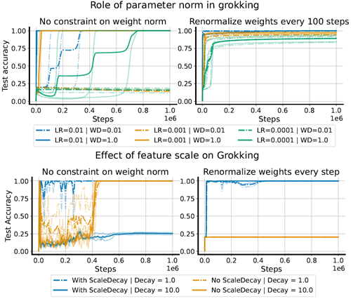
Figure 2: LHS: grokking occurs in networks whose updates induce nontrivial changes in the learned features, a
property which requires a sufficiently large update norm relative to the parameters. This can be achieved by increasing the learning rate or decreasing the parameter norm via weight decay, where a larger weight decay can compensate for a smaller learning rate and vice versa. Periodically re-scaling the parameters to their original norm thus blunts the effect of weight decay. RHS: when we add layer normalization to the network, a large ELR is not sufficient to induce grokking. Instead, it becomes necessary to also reduce the norm of the attention head inputs, which we achieve by applying weight decay to the scale parameters of the layernorm transforms in the network.
図2:LHS:グロッキングは、更新によって学習済みの特徴に重大な変化が生じるネットワークで発生します。この特性には、パラメータに対して十分に大きな更新ノルムが必要です。これは、学習率を上げるか、重み減衰によってパラメータノルムを減少させることで実現できます。重み減衰が大きいほど学習率が小さくなることを補うことができ、その逆も同様です。パラメータを定期的に元のノルムに再スケーリングすることで、重み減衰の影響を弱めることができます。RHS:ネットワークにレイヤー正規化を追加すると、大きなELRだけではグロッキングを誘発するのに十分ではありません。代わりに、アテンションヘッド入力のノルムも減らす必要があり、これはネットワーク内のレイヤーノルム変換のスケールパラメータに重み減衰を適用することで実現します。
While a high effective learning rate is one mechanism by which networks achieve feature learning, inducing feature-learning dynamics alone, for example by moving from one poorly generalizing solution to another, is not sufficient to achieve good test set performance. In the right subplot of Figure 2 we provide an example of this situation by adding layer normalization to the network architecture. Despite following an otherwise identical experimental protocol, we obtain wildly different results: in this new architecture, weight normalization completely fails to generalize. The reason for this is subtle: the layer normalization transform rescales the attention inputs to be much larger than they would be under the default weight initialization, and as a result the attention matrices have much lower entropy and are more difficult to optimize (Wortsman et al., 2023). If the network is able to modulate the parameter norm, it can increase the smoothness of the attention mask by reducing the norm of the key and query matrix parameters; the projected network has no such means of escape. However, if we apply a weight decay term to the scale parameters of the normalization layers,a technique which we refer to as which we refer to by the term ‘scale decay’, we obtain the blue curves on the right hand side of Figure 2. We thus conclude that generalization requires both meaningful changes to the learned representation, and a suitable loss landscape in which these changes converge to a smooth, generalizing
solution.
高い実効学習率はネットワークが特徴学習を達成するメカニズムの一つですが、例えば汎化の低い解から別の解へと移行するなど、特徴学習ダイナミクスを誘導するだけでは、良好なテストセット性能を達成するには不十分です。図2の右側のサブプロットは、ネットワークアーキテクチャに層正規化を追加することで、この状況の例を示しています。他の点では同一の実験プロトコルに従っているにもかかわらず、大きく異なる結果が得られます。この新しいアーキテクチャでは、重みの正規化は完全に汎化に失敗します。その理由は微妙です。層正規化変換は、アテンション入力をデフォルトの重み初期化よりもはるかに大きく再スケールするため、結果としてアテンション行列のエントロピーが大幅に低下し、最適化がより困難になります(Wortsman et al., 2023)。ネットワークがパラメータノルムを調整できる場合、キー行列とクエリ行列のパラメータのノルムを低減することでアテンションマスクの滑らかさを高めることができますが、射影されたネットワークにはそのような回避手段がありません。しかし、正規化層のスケールパラメータに重み減衰項を適用すると(この手法を「スケール減衰」と呼びます)、図2の右側にある青い曲線が得られます。したがって、一般化には、学習した表現への意味のある変更と、これらの変更が滑らかで一般化された解に収束する適切な損失ランドスケープの両方が必要であると結論付けられます。
Having identified the importance of the effective learning rate in grokking, we now explore how it can be manipulated to accelerate the onset of generalization. In order to achieve generalization, the optimization process much satisfy two criteria. First, the optimizer must spend sufficient time in a regime where nontrivial updates are being made to the network. Second, once generalization is achieved the learning rate should be reduced to improve stability and In Figure 3 we apply the protocol which generated the blue line of the rightmost subplot of Figure 2: we train a transform
with weight projection, layer normalization, and scale decay. In particular, by increasing the effective learning rate to a sufficiently large value via linear warmup and then following a cosine decay schedule, we rapidly obtain perfect test accuracy which persists even after one million optimizer steps.
グロッキングにおける実効学習率の重要性を特定したので、次に、一般化の開始を加速するために実効学習率を操作する方法を検討します。一般化を達成するためには、最適化プロセスが2つの基準を満たす必要があります。第1に、最適化プログラムは、ネットワークに重要な更新が行われている状態で十分な時間を費やす必要があります。第2に、一般化が達成されたら、安定性を向上させるために学習率を下げる必要があります。図3では、図2の右端のサブプロットの青い線を生成したプロトコルを適用します。つまり、重み投影、レイヤーの正規化、スケール減衰を使用して変換をトレーニングします。特に、線形ウォームアップによって実効学習率を十分に大きな値に増加させ、その後コサイン減衰スケジュールに従うことで、100万ステップの最適化後でも維持される完璧なテスト精度を迅速に実現します。
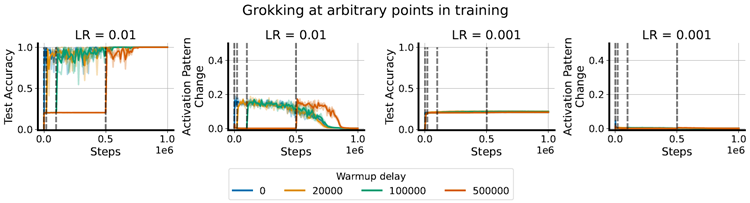
Figure 3: We can induce grokking at arbitrary points during training using targeted increases in the effective learning rate (timesteps where a learning rate increase occurs are denoted by dotted lines). This approach requires that the learning rate increase be sufficient to move feature learning metrics such as the percentage change in activation patterns in the network – we see in the LHS that increasing the learning rate to 0.01 leads to feature learning and grokking, whereas on the RHS 0.001 does not.
図3:実効学習率を意図的に増加させることで、訓練中の任意の時点でグロッキングを誘発することができます(学習率の増加が発生するタイムステップは点線で示されています)。このアプローチでは、学習率の増加が、ネットワーク内の活性化パターンのパーセンテージ変化などの特徴学習指標を変動させるのに十分なレベルである必要があります。左辺では、学習率を0.01に増加させると特徴学習とグロッキングが起こりますが、右辺では0.001では起こらないことがわかります。
An important difference between the typical setting for grokking and the continual learning settings which we will next investigate is that the modular arithmetic problem is stationary, and while we have shown how to accelerate grokking, have not shown that it is possible to induce grokking at arbitrary points in the learning process. It is plausible that the process by which features are learned depends crucially in some way on changes which our approach makes during the earliest phase of training. Figure 3 addresses this concern. We consider a range of increasingly long offsets, during which training at a learning rate too low to induce grokking occurs. After the desired interval, we then ‘turn on’ the learning rate schedule and proceed with training as normal. We observe that even after several hundred thousand optimizer steps, it is still possible to induce grokking via ELR re-warming.
グロッキングのための一般的な設定と、次に調査する継続学習設定との重要な違いは、モジュラー算術問題が定常であり、グロッキングを加速する方法を示したものの、学習プロセスの任意の時点でグロッキングを誘発できることを示していないことです。特徴を学習するプロセスは、トレーニングの初期段階で私たちのアプローチが行う変更に何らかの形で大きく依存していると考えられます。図 3 は、この懸念を示しています。グロッキングを誘発するには低すぎる学習率でのトレーニングが行われる、徐々に長くなるオフセットの範囲を検討します。必要な間隔が経過したら、学習率スケジュールを「オン」にして、通常どおりトレーニングを続行します。数十万の最適化ステップの後でも、ELR の再加温によってグロッキングを誘発できることが分かります。
We now explore whether ELR re-warming can also facilitate feature-learning, and hence generalization, in a different neural network architecture, data modality, and training regime: warm-starting image classifier training. Whereas a random initialization is designed to be relatively easy to overwrite, in this new setting the network must learn to overwrite previously learned features, a task which has the potential to be significantly more difficult than the grokking regime studied previously.
我々は今回、ELRリウォーミングが、異なるニューラルネットワークアーキテクチャ、データモダリティ、そして学習環境、すなわちウォームスタート画像分類器学習においても、特徴学習、ひいては汎化を促進できるかどうかを検証する。ランダム初期化は比較的容易に上書きできるよう設計されているが、この新しい設定では、ネットワークは以前に学習した特徴を上書きすることを学習する必要があり、これはこれまで研究されてきたグロッキング環境よりもはるかに困難となる可能性がある。
Experiment details. In this section, all experiments are run with convolutional architectures on the CIFAR-10 dataset. Denoting this dataset Dtotal, we expand on the protocol of Ash & Adams (2020) by first training the network on some subset Dinit which contains a randomly sampled subset of the data points in Dtotal. After a fixed interval of 70 epochs, the remainder of the dataset is added to Dinit, and the network continues training on the full dataset for another 70 epochs. We track test accuracy throughout the entire procedure. As a baseline, we include one setting where we “pretrain” on 100% of the training data, which presents an upper bound on the expected performance improvement from our approach.
実験の詳細 このセクションでは、CIFAR-10 データセットに対して畳み込みアーキテクチャを用いてすべての実験を実行します。このデータセットを Dtotal とし、Ash & Adams (2020) のプロトコルを拡張し、まず Dtotal 内のデータポイントのランダムにサンプリングされたサブセットを含むサブセット Dinit でネットワークをトレーニングします。70 エポックの固定間隔の後、データセットの残りが Dinit に追加され、ネットワークはさらに 70 エポックの間、完全なデータセットでトレーニングを続けます。手順全体を通してテスト精度を追跡します。ベースラインとして、トレーニングデータの 100% で「事前トレーニング」する設定を 1 つ含めています。これは、このアプローチによって期待されるパフォーマンス向上の上限を示します。
The Shrink and Perturb method (Ash & Adams, 2020) is a popular means of improving generalization on non-
stationary tasks (Schwarzer et al., 2023). This approach, which involves rescaling the parameters by a constant \(0\lt α\lt 1\) and then sampling a perturbation from the initialization distribution, can be viewed as a means of reducing the difficulty of escaping the local basin of the loss landscape at the current learning rate. Similar observations have been made theoretically in non-stationary online convex optimization, where the “effective diameter” of the active parameter space determines how quickly one can adapt to new data distributions and, among others, similar techiques are used to control the diameter (see, e.g., Gy¨orgy & Szepesv´ari, 2016). We propose to instead escape from a local minimum not by changing the loss landscape, but by increasing the learning rate, for example to a value which exceeds the sharpness of the local basin (Lewkowycz et al., 2020), so that the optimizer has the chance to jump out of the current basin. In Figure 4, we test whether ELR re-warming can close the generalization gap that emerges in warm-started neural networks, following the procedure outlined above (additional details can be found in Appendix A.2). We use five random seeds on three initial dataset fractions, corresponding to 10%, 50%, and 100% of the whole dataset. We track both notions of feature learning described in Equations 3 and 4, and observe that while the update norm for both training setups is similar in both iterations of training, the NaP variant applies more significant changes to the learned representation particularly in the second iteration, and attains the same final generalization performance independent of the initial dataset size.
Shrink and Perturb法(Ash & Adams, 2020)は、非定常タスクにおける一般化を向上させるための一般的な手法です(Schwarzer et al., 2023)。このアプローチは、パラメータを定数 \(0\lt α\lt 1\) で再スケーリングし、初期化分布から摂動をサンプリングするもので、現在の学習率で損失ランドスケープの局所的な盆地から脱出する困難さを軽減する手段と見なすことができます。同様の観察は、非定常オンライン凸最適化においても理論的に行われており、アクティブパラメータ空間の「有効直径」によって、新しいデータ分布にどれだけ速く適応できるかが決定され、直径を制御するために同様の手法が使用されています(例えば、Gy¨orgy & Szepesv´ari, 2016を参照)。我々は、損失ランドスケープを変更するのではなく、学習率を、例えば局所的領域 (Lewkowycz et al., 2020) の鋭さを超える値に増加させることで、最適化プログラムが現在の領域から抜け出す機会が得られるようにすることで、局所最小値から脱出することを提案する。図4では、上で概説した手順に従って、ウォームスタートしたニューラルネットワークで発生する一般化ギャップをELRの再ウォーミングによって埋めることができるかどうかをテストしている(詳細は付録A.2を参照)。データセット全体の10%、50%、100%に相当する3つの初期データセット部分に5つのランダムシードを使用する。式3と式4で説明した特徴学習の両方の概念を追跡し、両方のトレーニングセットアップの更新ノルムは両方のトレーニング反復で同様である一方、NaPバリアントは、特に2回目の反復で学習済み表現にさらに大きな変更を適用し、初期データセットサイズに関係なく同じ最終的な一般化パフォーマンスを達成することを観察する。
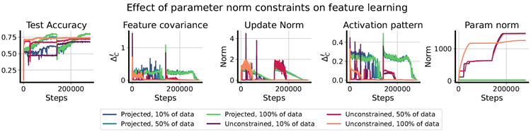
Figure 4: Learning rate re-warming on networks whose parameter norm is constrained so as to not grow significantly over the course of training exhibit significant improvements on CIFAR-10 over naively applying learning rate cycling on an unregularized network. We observe that feature-learning measures increase and then decline with each learning rate cycle in tandem with the learning rate. Although it applies similar update norms to the parameters, the unconstrained network exhibits notably less feature-learning in the second iteration by both the feature covariance and activation pattern metrics.
図4:パラメータノルムが訓練中に大きく増加しないように制約されたネットワークにおいて、学習率リウォーミングを行うと、正則化されていないネットワークに学習率サイクリングを単純に適用した場合と比較して、CIFAR-10において大幅な改善が見られる。特徴学習指標は学習率サイクルごとに増加し、その後減少する様子が見られる。パラメータに同様の更新ノルムを適用しているにもかかわらず、制約のないネットワークでは、特徴共分散と活性化パターンの両方の指標において、2回目の反復で特徴学習が著しく減少していることがわかる。
In the rightmost plot of Figure 5 we ablate the two critical components of the adaptive re-warming process: the use of weight projection to prevent unwanted decay in the effective learning rate over time, which would reduce the ability of the network to change its learned representation, and the use of a changepoint detection algorithm (for example the Cusum algorithm, Page, 1954) on the loss value to identify non-stationarities in the data-generating distribution which merit a learning rate reset. We show that removing any single component of this approach degrades performance, with the unconstrained parameters trained on a single continuous learning rate decay performing worst. We further show in Appendix B.2 that these results are also achieved when the fixed schedule does not align with the task change.
図5 の右端のプロットでは、適応型再加温プロセスの 2 つの重要な要素を省略しています。1 つは重み投影を使用して、有効学習率が時間の経過とともに望ましくない低下 (学習した表現を変更するネットワークの能力が低下する) を防ぐこと、もう 1 つは損失値に対する変化点検出アルゴリズム (たとえば、Cusum アルゴリズム、Page、1954) を使用して、学習率のリセットを必要とするデータ生成分布の非定常性を識別することです。このアプローチの 1 つの要素を削除するとパフォーマンスが低下し、単一の連続学習率低下でトレーニングされた制約のないパラメーターのパフォーマンスが最悪になることがわかります。さらに、付録 B.2 では、固定スケジュールがタスクの変更と一致しない場合にもこれらの結果が得られることを示しています。
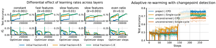
Figure 5: LHS: per-layer learning rate scaling. Re-scaling learning rates in different layers results in significant changes in the magnitude of the warm-starting effect. Intriguingly, while conditions with a higher absolute number
of dead neurons exhibit larger warm-starting effects, observing a higher relative number of dead units in networks warm-started from smaller datasets does not indicate that there will be a large generalization gap. RHS: using the CUSUM changepoint detection algorithm to determine when to re-warm the learning rate successfully closes the generalization gap in the warm-starting experiment regime; however, to gain the full benefits of learning rate rewarming, the parameter norm must be prevented from growing during the initial learning phase.
図5: LHS: 層ごとの学習率のスケーリング。 異なる層で学習率を再スケーリングすると、ウォームスタート効果の大きさに大きな変化が生じます。興味深いことに、デッドニューロンの絶対数が多い条件ではウォームスタート効果が大きくなりますが、より小さなデータセットからウォームスタートされたネットワークでデッドユニットの相対数が多いことが観察されても、大きな汎化ギャップが生じるとは限りません。RHS: CUSUM変化点検出アルゴリズムを使用して学習率の再ウォームアップのタイミングを決定することで、ウォームスタート実験における汎化ギャップをうまく解消できます。ただし、学習率の再ウォームアップのメリットを最大限に得るには、初期学習フェーズでパラメータノルムの増加を防ぐ必要があります。
Whereas the transformer architectures we considered in Section 4 consisted of a single attention layer, the deeper vision
architectures allow us to investigate whether different layers might exhibit different dynamics which benefit from
distinct learning rates. Prior work suggests that different layers in vision networks can exhibit distinct dynamics (Zhang
et al., 2021) and train optimally at distinct learning rates (Everett et al., 2024). While these findings are most applicable
to networks far larger than the ones we consider in this work, we conduct a preliminary investigation to gauge the utility
of layer-specific learning rates in maintaining plasticity, whose results we present in the LHS of Figure 5. We consider
four different per-layer learning rate assignments: a constant assignment, where every layer is given the same learning
rate; fast features, where the final linear layer’s learning rate is divided by 10; the analogous slow features, where
the non-final layers’ learning rates are divided by 10; and even-ratio-abs, which scales the learning rate of each layer
proportional to the average magnitude of the parameters, so that updates applied to each layer correspond to a constant
proportion of the layer’s L1 norm. The choice to distinguish between the final layer and all prior layers in two of
these assignments is due to the previously observed importance of the final layer scale in facilitating grokking in some
vision tasks (Liu et al., 2022b). We find that provided the learning rate on the features component of the network
is held constant, the learning rate on the final linear layer does not have a noticeable effect on performance at the
magnitudes we evaluated.
セクション 4 で検討したトランスフォーマー アーキテクチャは単一の注意層で構成されていましたが、より深いビジョン アーキテクチャでは、異なる層が異なるダイナミクスを示し、異なる学習率の恩恵を受けるかどうかを調査できます。先行研究では、ビジョン ネットワーク内の異なる層が異なるダイナミクスを示し (Zhang 他、2021)、異なる学習率で最適に学習できることが示唆されています (Everett 他、2024)。これらの知見は、本研究で検討するネットワークよりもはるかに大規模なネットワークに最も当てはまりますが、可塑性を維持する上での層固有の学習率の有用性を測定するための予備調査を実施し、その結果を図 5 の左側に示します。層ごとに 4 つの異なる学習率割り当てを検討します。定数割り当てでは、すべての層に同じ学習率が与えられます。高速特徴では、最終線形層の学習率が 10 で割られます。類似の低速特徴では、最終層以外の層の学習率が 10 で割られます。そしてeven-ratio-absは、各層の学習率をパラメータの平均値に比例してスケーリングし、各層に適用される更新が層のL1ノルムの一定の割合に対応するようにします。これらの課題のうち2つで最終層とそれ以前のすべての層を区別することを選択したのは、最終層のスケールが一部の視覚タスクにおけるグロッキングを促進する上で重要であることが以前に観察されているためです(Liu et al., 2022b)。ネットワークの特徴コンポーネントの学習率が一定に保たれている場合、最終線形層の学習率は、評価した大きさではパフォーマンスに顕著な影響を与えないことがわかりました。
Reinforcement learning presents a particularly challenging non-stationary learning problem due to the pathological dynamics induced by bootstrapping (Van Hasselt et al., 2018), the nonstationarity in the input observations as the state-visitation distribution evolves, and nonstationarity in the prediction target as a result of policy improvement (Lyle et al., 2022). While this nonstationarity makes RL a promising candidate to benefit from methods which accelerate feature-learning, its notoriety for instability and divergence (Ghosh & Bellemare, 2020) means that any attempt to increase the volatility of the learning dynamics, as we have sought in our ELR re-warming strategies, must be undertaken with care. In particular, we must ensure that by accelerating the rate at which the network changes its learned representation, we do not also accelerate its divergence or collapse before a good policy can be learned. We conjecture that learning rate cycling might therefore be particularly well-suited to reinforcement learning. By periodically increasing (re-warming) the learning rate, we aim to overwrite spurious correlations which interfere with policy improvement, and by then annealing the learning rate to a stable value we can avoid the instabilities that so often plague RL algorithms. We include additional details on the experiments conducted in this section in Appendix A.3.
強化学習は、ブートストラップによって引き起こされる病的なダイナミクス (Van Hasselt et al., 2018)、状態訪問分布の進化に伴う入力観測値の非定常性、およびポリシー改善の結果としての予測ターゲットの非定常性 (Lyle et al., 2022) により、特に困難な非定常学習問題を提示します。この非定常性により、RL は特徴学習を加速する手法の恩恵を受ける有望な候補となりますが、不安定性と発散で悪名高い (Ghosh & Bellemare, 2020) ため、ELR 再加温戦略で追求してきたように、学習ダイナミクスのボラティリティを高める試みは慎重に行う必要があります。特に、ネットワークが学習した表現を変更する速度を加速することで、適切なポリシーを学習する前に、ネットワークの発散や崩壊も加速しないようにする必要があります。したがって、学習率サイクリングは強化学習に特に適しているのではないかと推測しています。学習率を定期的に増加(リウォーミング)することで、方策の改善を妨げる偽の相関関係を上書きし、その後学習率を安定した値にアニーリングすることで、強化学習アルゴリズムにしばしば見られる不安定性を回避することを目指しています。このセクションで実施した実験の詳細については、付録A.3に記載しています。
We begin our investigation by considering cyclic learning rates in two different training regimes: a high update-to-data (UTD) ratio or data-efficient regime where the environment and learner take steps in tandem, and the low update-todata ratio or online regime, where the environment takes four steps per every learner update step. The data-efficient regime, which often uses much higher ratios of learner updates to environment steps than that considered in this paper, is notoriously prone to over-estimation bias and feature collapse, particularly when the training algorithm uses bootstrapping, and benefits significantly from a variety of resetting strategies. By contrast, the online regime tends to be more stable and benefits less if at all from parameter resets. Because learning rate re-warming bears many similarities to resets, we conjecture that it should provide a greater benefit in the high UTD regime. We test these hypotheses with a DQN (Mnih et al., 2015) and a Rainbow agent (Hessel et al., 2018) in the arcade learning environments (ALE) (Bellemare et al., 2013) with our results presented in Figure 6.
我々は調査を、環境と学習者が連携してステップを踏む高データ更新(UTD)比率またはデータ効率の高い体制と、環境が学習者の更新ステップごとに 4 ステップを踏む低データ更新比率またはオンライン体制の 2 つの異なるトレーニング体制における巡回学習率を考慮することから始めます。この論文で検討されているものよりも環境ステップに対する学習者更新の比率をはるかに高くすることが多いデータ効率の高い体制は、特にトレーニング アルゴリズムがブートストラッピングを使用する場合に、過大評価バイアスと特徴の崩壊を起こしやすいことで有名であり、さまざまなリセット戦略から大きなメリットを得ています。対照的に、オンライン体制はより安定している傾向があり、パラメーター リセットによるメリットは、あっても少なくなります。学習率の再加温はリセットと多くの類似点があるため、高 UTD 体制でより大きなメリットをもたらすと推測されます。私たちはこれらの仮説をアーケード学習環境 (ALE) (Bellemare et al., 2013) の DQN (Mnih et al., 2015) と Rainbow エージェント (Hessel et al., 2018) を使用してテストし、その結果を図 6 に示します。
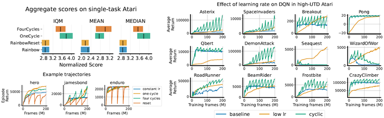
Figure 6: LHS: Cycling the learning rate in a Rainbow agent with weight projection trained in a low update-todata regime exhibits heterogeneous effects across environments, outperforming resets and a constant learning rate but exhibiting similar performance to a single cycle of learning rate decay. Agents recover faster from learning rate rewarming than from resets. RHS: Cyclic learning rates produce much more pronounced effects in DQN under a high replay ratio, outperforming both fixed learning rate baselines in several environments, but sometimes suffers from instability in environments like Seaquest and Wizard of Wor.
図6:左:低データ更新モードで訓練された重み投影を用いたRainbowエージェントにおいて、学習率を循環させると、環境間で異質な効果が現れ、リセットや一定学習率よりも優れたパフォーマンスを示すものの、学習率減衰の単一サイクルと同等のパフォーマンスを示す。エージェントは、リセットよりも学習率の再加温からより速く回復する。右:循環学習率は、高再生率のDQNにおいてより顕著な効果を発揮し、いくつかの環境で固定学習率ベースラインの両方を上回るパフォーマンスを示すが、SeaquestやWizard of Worのような環境では不安定になることがある。
Low UTD regime We observe heterogeneous effects from learning rate cycling across environments in the LHS subplot of Figure 6, where we present results for Rainbow agents trained with NaP. While the resulting performance curves from cyclic learning rates exhibit some similarity to those attained by resets in that both exhibit an initial performance drop, the cyclic LR agent recovers more rapidly and attains higher final performance on most environments. We tend to see convergence of the cyclic schedules to approximately the same performance at the end of training regardless of the number of cycles applied, suggesting that the benefits of these approaches can be attributed largely to spending sufficient time at key learning rates rather than exposing the network to higher ELRs later in training.
低 UTD 体制 図 6 の LHS サブプロットでは、環境間での学習率サイクリングによる異質な効果が見られます。ここでは、NaP でトレーニングされた Rainbow エージェントの結果を示しています。循環学習率から得られるパフォーマンス曲線は、どちらも初期のパフォーマンスの低下を示すという点でリセットによって達成されるものといくらか類似していますが、循環 LR エージェントはより急速に回復し、ほとんどの環境でより高い最終パフォーマンスを達成します。適用されたサイクル数に関係なく、トレーニングの最後には循環スケジュールがほぼ同じパフォーマンスに収束する傾向があります。これは、これらのアプローチの利点が、トレーニングの後半でネットワークをより高い ELR にさらすのではなく、主要な学習率で十分な時間を費やすことに主に起因することを示唆しています。
High UTD regime Whereas in the low UTD regime performance of all methods frequently converged to the same final value, we see much greater variability in score in the high-UTD regime, largely due to the instability of larger learning rates. We evaluate two different learning rates on a DQN agent trained without weight decay or projection, where the baseline value is trained at a constant learning rate of 6.25e-5, while the low lr variant trains with a constant step size of 1e-6, along with a cyclic variant that oscillates between the two values. While the cyclic variant often exhibits performance improvements, it suffers from similar degrees of instability in environments such as seaquest and krull as the higher learning rate variant. In the next section, we will investigate a means of mitigating this instability.
高 UTD 状態 低 UTD 状態ではすべての手法のパフォーマンスが同じ最終値に収束することが多いのに対し、高 UTD 状態ではスコアの変動がはるかに大きくなります。これは主に学習率が高い場合の不安定性によるものです。重み減衰や投影なしでトレーニングした DQN エージェントで 2 つの異なる学習率を評価します。ベースライン値は 6.25e-5 の一定学習率でトレーニングされ、低 lr バリアントは 1e-6 の一定ステップ サイズでトレーニングされ、2 つの値の間を振動する巡回バリアントもあります。巡回バリアントはパフォーマンスが向上することがよくありますが、seaquest や krull などの環境では、高学習率バリアントと同程度の不安定性に悩まされます。次のセクションでは、この不安定性を軽減する手段を調査します。
While LR cycling improves performance in some environments in the high-UTD regime, it is clear that in many environments optimal performance requires extended periods of low-learning-rate training. These difficulties can in large part be attributed to the nature of the environments on which we evaluate: reinforcement learning agents tend to experience greater non-stationarity at the beginning of training, and also tend to see significant performance improvements from the low-learning-rate phase of an ELR cycle than would be expected in supervised learning (Lyle et al., 2024a). We therefore propose to perform early-stopping of the cyclic schedule, using a cycle period of 4M optimizer steps and switching to a constant learning rate after ten cycles of re-warming, or 40M frames, for the remainder of training. We observe similar results for other choices of stopping point in Appendix B.3. In Figure 7, we show that this approach results in consistent and dramatic performance improvements in both Rainbow and DQN agents trained in the high-UTD regime on Atari environments. We observe particularly significant improvements in seaquest and krull, two domains where the cyclic learning rate schedule struggled with instability. The early cycling of the learning rate results in improvements over the constant low learning rate, demonstrating the benefits of transiently passing through the high-LR regime (repeatedly). We show in Appendix B.3 that the DQN agent exhibits similar benefits from early-stopping at 8M or 20M frames.
LRサイクリングは、高UTD領域において一部の環境でパフォーマンスを向上させますが、多くの環境では最適なパフォーマンスを得るには、長期間の低学習率トレーニングが必要であることは明らかです。これらの困難は、主に評価対象となる環境の性質に起因しています。強化学習エージェントは、トレーニング開始時に非定常性が大きく、また、教師あり学習で期待されるよりも、ELRサイクルの低学習率フェーズから大幅なパフォーマンス向上が見られる傾向があります(Lyle et al., 2024a)。そこで、我々は、400万ステップの最適化ステップをサイクル期間として、サイクリングスケジュールを早期に停止することを提案します。そして、10サイクルの再ウォーミング(4000万フレーム)後に、残りのトレーニング期間で一定の学習率に切り替えます。付録B.3では、他の停止点の選択肢についても同様の結果が得られています。図7では、このアプローチにより、Atari環境において高UTD領域でトレーニングされたRainbowエージェントとDQNエージェントの両方で、一貫して劇的なパフォーマンス向上が達成されていることを示しています。特に、巡回学習率スケジュールが不安定さに悩まされていた2つの領域、SeaQuestとKrullにおいて顕著な改善が見られました。学習率の早期巡回は、一定の低い学習率の場合よりも改善が見られ、高LR領域を一時的に(繰り返し)通過することの利点を示しています。付録B.3では、DQNエージェントが8Mフレームまたは20Mフレームで早期停止することで同様の利点を示すことを示しています。
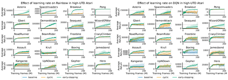
Figure 7: DQN and Rainbow agents both benefit from early learning rate cycling followed by annealing in high-UTD
Atari settings, with significant improvements over the constant and continual cyclic learning rates.
図7:DQNエージェントとRainbowエージェントはどちらも、早期学習率サイクリングとそれに続く高UTD Atari設定でのアニーリングの恩恵を受けており、一定および継続的な循環学習率に比べて大幅な改善が見られます。
This work has shown that re-warming of the effective learning rate can rapidly induce feature-learning, and thus generalization, in a variety of neural network training tasks. We proposed a simple modification to the Normalize-and-Project method which introduces a non-monotone learning rate schedule and used this approach to facilitate grokking, that is, to overwrite initial features which permitted memorization of the training data with ones that generalize. We further showed that the same ELR re-warming techniques designed to facilitate grokking can just as readily be applied to overwrite learned features, demonstrating the efficacy of learning rate re-warming at closing the generalization gap induced by warm-starting neural network training. We further observed significant improvements from learning rate re-warming in high-update-to-data reinforcement learning tasks, though we observe much greater instability at high learning rates which requires more aggressive annealing than was required in classification tasks. We conclude that re-warming the effective learning rate is a powerful tool for combating primacy bias in neural networks, but that it must be deployed with care to avoid introducing instabilities which can derail the feature-learning process which it was intended to facilitate.
本研究では、実効学習率の再加温により、様々なニューラルネットワークトレーニングタスクにおいて、特徴学習、ひいては一般化が急速に促進されることを示した。我々は、非単調な学習率スケジュールを導入する正規化・投影法の単純な修正を提案し、この手法を用いてグロッキング(grokking)を促進、すなわちトレーニングデータの記憶を可能にする初期特徴を一般化可能な特徴で上書きすることを可能にした。さらに、グロッキングを促進するために設計された同じELR再加温手法が、学習済み特徴の上書きにも容易に適用できることを示し、ウォームスタートによるニューラルネットワークトレーニングによって誘発される一般化ギャップを埋める上で、学習率の再加温の有効性を実証した。さらに、データ更新頻度の高い強化学習タスクにおいて、学習率の再加温によって顕著な改善が見られることを確認したが、高学習率では不安定性が大幅に増大し、分類タスクで必要とされるよりも積極的なアニーリングが必要となることがわかった。実効学習率の再調整は、ニューラル ネットワークにおけるプライマシー バイアスに対抗する強力なツールであるが、促進することを目的とした特徴学習プロセスを狂わせる可能性のある不安定性を導入しないように注意して導入する必要があるという結論に達しました。
\[ \boxed{ \begin{array}{c|c} \textbf{Parameter} & \textbf{Value} \\ \hline \text{num layers} & 2 \\ \hline \text{num heads} & 4 \\ \hline \text{query/key/value dimension} & 32 \\ \hline \text{feed-forward hidden size} & 512 \\ \hline \text{dropout rate} & 0 \\ \hline \text{relative position embeddings} & \text{False} \\ \hline \text{absolute position length} & 5 \\ \hline \text{LayerNorm position} & \text{before attention, before MLP, after MLP} \end{array} } \]
Architecture details we provide details on the transformer architecture in Table 1. The architecture consists of an input embedding layer using absolute positional encoding, followed by a single attention block, followed by a two-layer MLP, followed by a decoding layer. LayerNorm layers, when incorporated, are applied to the attention inputs and outputs, and the MLP outputs. We omit bias terms in the network and use RMSNorm by default.
アーキテクチャの詳細 表1にTransformerアーキテクチャの詳細を示します。このアーキテクチャは、絶対位置エンコーディングを用いた入力埋め込み層、単一のアテンションブロック、2層MLP、デコード層で構成されています。LayerNorm層が組み込まれている場合は、アテンション入力と出力、およびMLP出力に適用されます。ネットワークではバイアス項を省略し、デフォルトでRMSNormを使用します。
Training protocols In all experiments, we use an Adam optimizer with variable step size and default values for \(β_1=0.9,β_2 =0.999\). The dataset is constructed as described in the main body of the paper. The learning rate schedules we consider are a constant learning rate and a cosine warmup learning rate schedule with 1000 warmup steps and a final learning rate of 0.0001. One important note on our division of the dataset into a training and testing subset is that pairs \((x, y)\) and \((y, x)\) are not distinguished, meaning that a network which has learned to treat its inputs symmetrically but has not learned any other generalizing features will attain approximately 20% accuracy on the test set via this symmetry. This observation casts an intriguing light on the results of Figure 2, where we sometimes see networks drop below this 20% threshold prior to grokking.
トレーニング プロトコル すべての実験では、可変ステップ サイズとデフォルト値 \(β_1=0.9,β_2 =0.999\) を持つ Adam 最適化ツールを使用します。データセットは、論文の本文で説明されているとおりに構築されています。検討する学習率スケジュールは、一定の学習率と、ウォームアップ ステップが 1000 ステップで最終学習率が 0.0001 であるコサイン ウォームアップ学習率スケジュールです。データセットをトレーニング用とテスト用のサブセットに分割する際の重要な注意点は、ペア \((x, y)\) と \((y, x)\) は区別されないことです。つまり、入力を対称的に扱うことを学習したが、他の一般化機能を学習していないネットワークは、この対称性によりテスト セットで約 20% の精度を達成します。この観察は、図 2 の結果に興味深い光を当てます。図 2 では、ネットワークが理解する前にこの 20% のしきい値を下回ることがあることがわかります。
In our warm-starting experiments we consider two similar network architectures: a ResNet18 architecture (He et al., 2015), and a smaller CNN based on a popular architecture for reinforcement learning (Mnih et al., 2015). We use an adam optimizer with variable step size and otherwise default hyperparameters. The sub-sampled dataset is selected by specifying the appropriate number of data points in the tfds.load function from the tensorflow datasets library.
ウォームスタート実験では、2つの類似したネットワークアーキテクチャ、すなわちResNet18アーキテクチャ(He et al., 2015)と、強化学習で広く使用されているアーキテクチャに基づく小規模なCNN(Mnih et al., 2015)を検討します。可変ステップサイズと、その他のハイパーパラメータはデフォルトのAdamオプティマイザーを使用します。サブサンプリングされたデータセットは、TensorFlowデータセットライブラリのtfds.load関数で適切なデータポイント数を指定することにより選択されます。
CNN architecture: for the CNN architecture, we apply three convolutional layers of 5x5, 3x3, and 3x3 kernels in
the first, second, and third layers respectively, each with 32 channels. Each convolutional layer is followed by a LayerNorm and then a ReLU nonlinearity. The convolutional outputs are then flattened and fed through a single hidden fully connected layer with a ReLU activation. We apply a linear layer to this output to obtain the prediction logits.
CNNアーキテクチャ: CNNアーキテクチャでは、第1層、第2層、第3層にそれぞれ5x5、3x3、3x3カーネルの3つの畳み込み層を適用し、各層は32チャネルです。各畳み込み層の後にはLayerNorm、そしてReLU非線形性が続きます。畳み込み出力は平坦化され、ReLU活性化を伴う単一の全結合隠れ層に入力されます。この出力に線形層を適用し、予測ロジットを取得します。
ResNet architecture: the ResNet is a standard ResNet-18 (He et al., 2015), with the only notable modification being that we do not include bias terms in the linear transforms, finding that they complicate the estimation of the effective
learning rate without improving performance of the model.
ResNetアーキテクチャ: ResNetは標準的なResNet-18(He et al., 2015)ですが、唯一の注目すべき変更点は線形変換にバイアス項を含めないことです。バイアス項はモデルのパフォーマンスを向上させることなく、実効学習率の推定を複雑にすることがわかりました。
High UTD regime We evaluated DQN and Rainbow on 20 games: Asterix, SpaceInvaders, Breakout, Pong, Qbert, DemonAttack, Seaquest, WizardOfWor, RoadRunner, BeamRider, Frostbite, CrazyClimber, Assault, Krull, Boxing, Jamesbond, Kangaroo, UpNDown, Gopher, and Hero. We used a reply ratio of 1 (four times the default value). The minimum and maximum learning rate of the cyclic schedule are 1e-6 and 6.25e-5, respectively. The cycle length is 4M environment step. For weight decay experiments, we used a value of 1e-2.
高UTDモード DQNとRainbowを20種類のゲーム(Asterix、SpaceInvaders、Breakout、Pong、Qbert、DemonAttack、Seaquest、WizardOfWor、RoadRunner、BeamRider、Frostbite、CrazyClimber、Assault、Krull、Boxing、Jamesbond、Kangaroo、UpNDown、Gopher、Hero)で評価しました。応答率は1(デフォルト値の4倍)を使用しました。巡回スケジュールの最小学習率は1e-6、最大学習率は6.25e-5です。巡回期間は4M環境ステップです。重み減衰実験では、1e-2の値を使用しました。
Low UTD regime We train a Rainbow agent on 57 games in the Arcade Learning Environment benchmark, following the protocol used by (Hessel et al., 2018). We use an adam optimizer with a default learning rate defaulting to 6.25e-5. Cyclic learning rates use this as their maximal value. Training occurs for 200M frames.
低UTDモード Arcade Learning Environmentベンチマークを用いて、Rainbowエージェントを57のゲームで学習させました。これは、Hesselら(2018)が使用したプロトコルに基づいています。学習率はAdamオプティマイザーを使用し、学習率はデフォルトで6.25e-5に設定されています。巡回学習率は、この値を最大値として使用します。学習は2億フレーム行われます。
We observe in the right-hand-side of Figure 8 that grokking consistently coincides with a reduction in the rank of
the attention head outputs, and that reducing the rank of these outputs in networks with layer normalization requires
reducing the norm of either the attention head inputs or the key and query matrices.
図8の右側を見ると、グロッキングはアテンションヘッド出力のランクの低下と一貫して一致しており、層の正規化を伴うネットワークでは、これらの出力のランクを下げるには、アテンションヘッド入力またはキー行列とクエリ行列のいずれかのノルムを下げる必要があることがわかります。
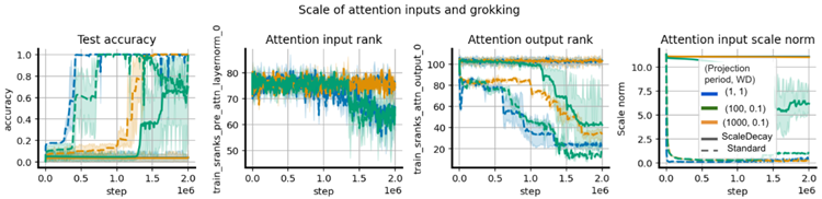
Figure 8: Relationship between attention output rank and grokking in networks trained with LayerNorm and periodic parameter renormalization. Grokking frequently coincides with a reduction in the rank of the attention outputs. Colours correspond to varying weight decay and projection frequency values.
図8: LayerNormと定期的なパラメータ再正規化を用いて学習したネットワークにおける、注意出力のランクとグロッキングの関係。グロッキングは、注意出力のランクの低下と頻繁に一致する。色は、重みの減衰と投影頻度の変化に対応している。
While it is important to give time for a cyclic learning rate to complete at least one full cycle after additional data has
been added in order to maximally benefit from learning rate re-warming, it is not necessary for this cycle to coincide
perfectly with the addition of new data. We replicate the experimental setting of Figure 4 but now set a cyclic learning
rate which re-warms 5 times throughout training, so that the new data is added half-way through the third cycle. We
see in Figure 9 that this setting also closes the generalization gap.
学習率の再ウォーミングから最大限の利益を得るには、追加データが追加された後、巡回学習率が少なくとも1サイクル完了するまでの時間を与えることが重要ですが、このサイクルが新しいデータの追加と完全に一致する必要はありません。図4の実験設定を再現しますが、今度は訓練中に5回再ウォーミングする巡回学習率を設定し、新しいデータが3サイクル目の途中で追加されるようにします。図9を見ると、この設定によって汎化ギャップも解消されていることがわかります。
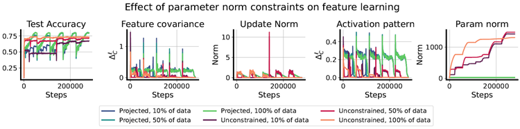
Figure 9: Replicating the results of Figure 4, we see that it is not necessary for the task boundary and ELR re-warming
period to align for generalization to benefit from the effects of ELR re-warming.
図9:図4の結果を再現すると、一般化がELR再加温の効果から利益を得るためには、タスク境界とELR再加温期間が一致する必要はないことがわかります。
The choice of when to switch from a cyclic learning rate to a constant low learning rate is somewhat arbitrary. Prior
work has observed that a longer low-learning-rate phase of training can be beneficial to agents in the Arcade Learning
巡回学習率から一定の低学習率に切り替えるタイミングの選択は、ある程度恣意的である。先行研究では、アーケード学習において、低学習率の訓練期間を長くすることがエージェントにとって有益となる可能性があることが観察されている。
Environment (Lyle et al., 2024a), but did not conduct a thorough sweep. We perform a coarse grid-search over three different stopping points for the learning rate cycling applied to the DQN agent in Figure 10, observing some variance in outcomes but qualitatively similar effects across all three stopping points when compared to a fixed learning rate.
環境(Lyle et al., 2024a)は、徹底的な調査は行いませんでした。図10のDQNエージェントに適用された学習率サイクリングについて、3つの異なる停止点において粗いグリッドサーチを実行したところ、結果には多少のばらつきが見られましたが、固定学習率と比較すると、3つの停止点すべてにおいて定性的に同様の効果が見られました。
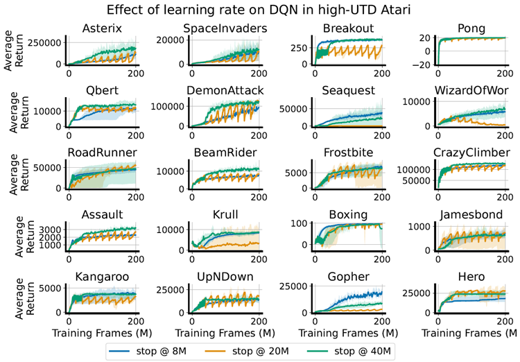
Figure 10: On average, running the cyclic learning rate schedule for longer before annealing results in slightly better
performance, but this improvement depends on the game and is not uniform.
図10: 平均すると、アニーリング前に巡回学習率スケジュールを長く実行すると、パフォーマンスがわずかに向上しますが、この改善はゲームによって異なり、均一ではありません。
In addition to the variants studied in the main body of the paper, we evaluate two additional variants in Figure 11: an early-stopping variant of the cyclic learning rate schedule which terminates at a final value of 1e-7 after three-quarters of the budget has elapsed, and a variant of the resetting agent that uses a cyclic learning rate schedule that aligns with the reset period. We include per-game results for the Rainbow agent trained in the low-update-to-data regime in Figure 12 for all 57 games.
本論文本文で検討したバリアントに加えて、図11ではさらに2つのバリアントを評価しています。1つは、予算の4分の3が経過した後に最終値1e-7で終了する巡回学習率スケジュールの早期終了バリアント、もう1つはリセット期間と一致する巡回学習率スケジュールを使用するリセットエージェントのバリアントです。図12には、データ更新が少ない状態でトレーニングされたRainbowエージェントの、全57ゲームにおけるゲームごとの結果を示しています。
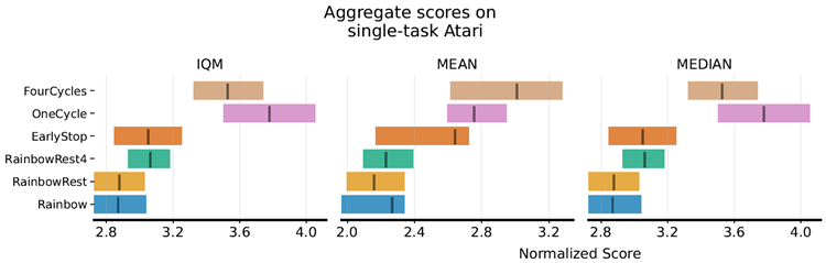
Figure 11: Additional variants on Atari. Early-stopping of the learning rate cycling to a very small learning rate (1e-7) does not improve performance (an exhaustive sweep of terminal values was not feasible due to the computational burden of the benchmark, so it is possible that a higher final value would perform better). Similarly, adding a cyclic learning rate schedule to the reset variant which matches the reset frequency improves performance over the constant learning rate variant but still leaves a large gap with the non-reset variants.
図11: Atariにおける追加のバリアント。学習率サイクルを非常に小さな学習率(1e-7)に早期停止しても、パフォーマンスは向上しません(ベンチマークの計算負荷のため、最終値を網羅的に掃引することは不可能であったため、最終値が高い方がパフォーマンスが向上する可能性があります)。同様に、リセット頻度に一致する周期的な学習率スケジュールをリセットバリアントに追加すると、一定学習率バリアントよりもパフォーマンスが向上しますが、リセットなしのバリアントとの差は依然として大きく残ります。
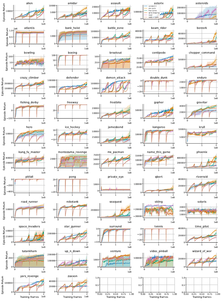
Figure 12: Results for low-UTD rainbow on all atari games.
図12: すべての Atari ゲームにおける低 UTD レインボーの結果。
In Figure 13 we also observe that under some of the per-layer learning rate schedules which do not alone close the warm-starting gap, it is possible to overcome this limitation by re-warming the learning rate to a larger value than what was used in the initial round of training. That is, in the setting considered here, it is necessary for the maximal ELR in the second iteration to exceed its maximal value in the first iteration. We demonstrate this finding in the right-hand-side plot of Figure 5, where we see that re-warming the learning rate to a value one order of magnitude above the initial learning rate produces the smallest generalization gaps. The effect of this larger re-warming value on the features can be seen by the sharp increase in rank attained by the larger relative re-warmed values compared to the network trained with identical learning rates.
図13 では、ウォーム スタート ギャップを単独では埋められないレイヤーごとの学習率スケジュールの一部では、学習率を最初のトレーニング ラウンドで使用された値よりも大きな値に再ウォーミングすることでこの制限を克服できることもわかります。つまり、ここで検討した設定では、2 回目の反復での最大 ELR が最初の反復での最大値を超える必要があります。この発見は図 5 の右側のグラフで示されており、学習率を初期学習率より 1 桁大きい値に再ウォーミングすると、一般化ギャップが最小になることがわかります。このより大きな再ウォーミング値が特徴に与える影響は、同一の学習率でトレーニングされたネットワークと比較して、より大きな相対的な再ウォーミング値によって達成される順位の急激な増加によって確認できます。
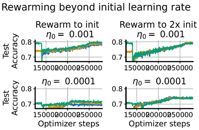
Figure 13: Under some conditions, fully closing the generalization gap requires re-warming the learning rate to a higher value than was used at the start of training – the small gap between networks trained at different initial data
fractions on the left column vanishes on the right after increasing the LR above the value used in the initial training phase.
図13: 状況によっては、一般化ギャップを完全に埋めるには、学習率をトレーニング開始時に使用した値よりも高い値に再加熱する必要があります。左側の列で異なる初期データ割合でトレーニングされたネットワーク間の小さなギャップは、LRを初期トレーニングフェーズで使用した値よりも高くすると、右側の列では消失します。
It is important to emphasize that our ability to induce feature learning depends not only on increasing the learning rate,
but ensuring that the parameter norm does not grow in tandem.
特徴学習を誘導する能力は、学習率を上げるだけでなく、パラメータノルムが連動して増加しないようにすることにも依存することを強調することが重要です。
Consider a single-hidden-layer neural network with ReLU activations, and m-dimensional input and a one-dimensional output, which can be written in the form
ReLU活性化関数とm次元入力と1次元出力を持つ、次のような形式で記述できる単一隠れ層ニューラルネットワークを考える。
\[
f(x)=w_2^T Relu(W_1x) \tag{5}
\]
where \(W_1∈\mathbb{R}^{m×d}, w_2∈\mathbb{R}^d, x∈\mathbb{R}^m\) and \(Relu(s)=max(s,0)\) is the ReLU function (when it is applied to a vector,
it is done coordinatewise).
ここで\(W_1∈\mathbb{R}^{m×d}, w_2∈\mathbb{R}^d, x∈\mathbb{R}^m\)および\(Relu(s)=max(s,0)\)はReLU関数です(ベクトルに適用される場合、座標ごとに行われます)。
We assume a simplified optimization setting with inputs \(\mathbf{X}∈\mathbb{R}^{n×m}\), where \(n\) denotes the number of data points and \(m\) the input dimension, so that each row of (\mathbf{X}\) is of the form \(\mathbf{x}_k\) for some data point \(\mathbf{x}_k∈\mathbb{R}^m\) . We will use the notation \(Φ=W_1\mathbf{X}\) to refer to pre-ReLU value of the network’s hidden features. We assume that gradients can be modeled as random Gaussian perturbations to the parameters. In particular, we assume the gradients on the first layer parameters
入力 \(\mathbf{X}∈\mathbb{R}^{n×m}\) を用いた簡略化された最適化設定を仮定する。ここで \(n\) はデータ点の数、 \(m\) は入力次元を表す。つまり、(\mathbf{X}\) の各行は、あるデータ点 \(\mathbf{x}_k∈\mathbb{R}^m\) に対して \(\mathbf{x}_k\) という形式となる。ネットワークの隠れ特徴の ReLU 前の値を参照するために、表記 \(Φ=W_1\mathbf{X}\) を使用する。勾配は、パラメータに対するランダムなガウス分布の摂動としてモデル化できると仮定する。特に、第 1 層のパラメータの勾配は
\(W_1\), denoted \(g∈\mathbb{R}^{m×d}\), follow the distribution \(g[i,j]\sim \mathcal{N}\left(0,\frac{σ_g^2}{d}\right)\) so that the expected norm for each row satisfies \(\mathbb{E}[||\mathbf{g}_i||]= σ_g^2\) (the Gaussian approximation holds when \(m\) is large enough and the network is close to initialization, as can be seen, e.g., from the form of the gradient in Equation (2.2) of Xu et al., 2024). We start with a simple question: how does the angle of an embedding \(Φ_k=W_1\mathbf{x}_k\) change as a function of the effective learning rate?
\(W_1\) は \(g∈\mathbb{R}^{m×d}\) と表記され、分布 \(g[i,j]\sim \mathcal{N}\left(0,\frac{σ_g^2}{d}\right)\) に従い、各行の期待ノルムは \(\mathbb{E}[||\mathbf{g}_i||]= σ_g^2\) を満たします(ガウス近似は \(m\) が十分に大きく、ネットワークが初期化に近い場合に成立します。これは、例えば、Xu et al., 2024 の式(2.2)の勾配の形からわかります)。まず、単純な疑問から始めます。埋め込み \(Φ_k=W_1\mathbf{x}_k\) の角度は、有効学習率の関数としてどのように変化するのでしょうか?
Consider the embedding of a single input, which we will denote \(Φ_k =W_1\mathbf{x}_k\). Then, after a single gradient update, we will have \(Φ_k^\prime=(W_1−η\mathbf{g})\mathbf{x}_k\). We assume that \(W_1\) has been initialized following the standard fan-in procedure, such that \(||W_1[i,:]||\approx 1\), that is, the Euclidean norm of each row of this parameter matrix is approximately 1. Straightforwardly, we have that the expected change in the angle \(θ\) between \(Φ_k\) and \(Φ_k^\prime\) grows as a function of the step size \(η\). In particular, assuming \(||η\mathbf{g}||=\sum_{i=1}^m η||\mathbf{g}_i||\approx ησ_g\sqrt{m}\) and that \(⟨\mathbf{g},W_1[i]⟩\approx 0\) (reasonable assumptions for sufficiently high-dimensional inputs), we have
単一の入力の埋め込みを考えてみましょう。これを \(Φ_k =W_1\mathbf{x}_k\) と表記します。そして、単一の勾配更新の後、\(Φ_k^\prime=(W_1−η\mathbf{g})\mathbf{x}_k\) となります。\(W_1\) は標準的なファンイン手順に従って初期化され、\(||W_1[i,:]||\approx 1\)、つまりこのパラメータ行列の各行のユークリッドノルムが約 1 であると仮定します。簡単に言うと、\(Φ_k\) と \(Φ_k^\prime\) の間の角度 \(θ\) の期待変化は、ステップサイズ \(η\) の関数として増大します。特に、\(||η\mathbf{g}||=\sum_{i=1}^m η||\mathbf{g}_i||\approx ησ_g\sqrt{m}\) と \(⟨\mathbf{g},W_1[i]⟩\approx 0\) (十分に高次元の入力に対する妥当な仮定)を仮定すると、
\[
\frac{⟨Φ_k,Φ_k^\prime⟩}{||Φ_k||||Φ_{k+1}||}\approx =\frac{1}{1+η^2σ_g^2} \tag{6}
\]
meaning that the rate at which the angle of the embedding changes depends on the learning rate. In a network which is scale-invariant with respect to the parameters of the first layer, i.e. where we have
つまり、埋め込みの角度が変化する速度は学習率に依存する。第1層のパラメータに関してスケール不変なネットワーク、すなわち、
\[
f(\mathbf{X})=2_2^T Relu\left(\frac{W_1\mathbf{X}}{||W_1\mathbf{X}||}\right)=w_2^T\tilde{Φ}
\]
then scaling \(W_1\) by a scalar \(α\) results in the expected rotation of the new features \(\tilde{Φ}^\prime\) obtained after applying a single
gradient descent step to \(W_1\)
そして、\(W_1\)をスカラー\(α\)でスケーリングすると、\(W_1\)に1回の勾配降下法を適用した後に得られる新しい特徴量\(\tilde{Φ}^\prime\)の期待回転が得られる。
\[
\mathbb{E}\left[\frac{\langle\tilde{Φ}_k,\tilde{Φ}_k^\prime\rangle}{||\tilde{Φ}_k||||\tilde{Φ}_k^\prime||}\right]\approx
\frac{1}{\sqrt{1+\frac{η^2}{α^2}σ_g^2}}
\]
where the approximation becomes tighter due to the orthogonality of gradients to parameters in scale-invariant functions.
ここで、スケール不変関数のパラメータに対する勾配の直交性により、近似はより厳密になります。
One can analogously estimate the probability, given a random initialization and a random update, that a currently-activated ReLU unit under some input will be deactivated after a single gradient step. In this case, we have \(Φ_{i,k} \sim \mathcal{N}(0,1)\) and – assuming \(||\mathbf{x}_k||=1–g_i^T\mathbf{x}_k\sim \mathcal{N}(0,σ_g^2)\), meaning that the update to \(Φ_{i,k}\) after a gradient step is a
Gaussian random variable \(\mathbf{z}\sim \mathcal{N}(0,η^2σ_g^2)\). The event we are interested in is thus
同様に、ランダムな初期化とランダムな更新が与えられた場合、ある入力の下で現在活性化されているReLUユニットが1回の勾配ステップ後に非活性化される確率を推定することができる。この場合、\(Φ_{i,k} \sim \mathcal{N}(0,1)\)となり、\(||\mathbf{x}_k||=1–g_i^T\mathbf{x}_k\sim \mathcal{N}(0,σ_g^2)\)と仮定すると、勾配ステップ後の\(Φ_{i,k}\)の更新はガウス分布確率変数\(\mathbf{z}\sim \mathcal{N}(0,η^2σ_g^2)\)となる。したがって、ここで注目する事象は以下の通りである。
\[
\begin{align}
P(Φ_{i,k}−\mathbf{z}\lt 0|Φ_{i,k}\gt 0) &=1−P(Φ_{i,k}−
\mathbf{z}\gt 0|Φ_{i,k}\gt 0) \\
\\
&=1-\left(\frac{1}{2}+\frac{1}{\pi}\arctan\frac{1}{\eta\sigma_g}\right) \\
\\
&=\frac{1}{2}-\frac{1}{\pi}\arctan\frac{1}{\eta\sigma_g}
\end{align}
\]
which holds for \(ησ_g ≤1\) following a derivation from Stackoverflow2. So the likelihood of a perturbation changing the activity of a particular unit scales as \(\arctan(\frac{1}{η})\), assuming our original (not scale-invariant) setup. Incorporating
scale-invariance means that now the likelihood of the activity of a particular neuron changing depends on the effective learning rate. In particular, supposing now that \(W_1\) is scaled by a factor \(α\), we obtain
これはStackoverflow2からの導出に従って、\(ησ_g ≤1\) の場合に成立する。したがって、特定のユニットの活動を変化させる摂動の確率は、元の(スケール不変ではない)設定を仮定すると、\(\arctan(\frac{1}{η})\) に比例する。スケール不変を考慮すると、特定のニューロンの活動が変化する確率は実効学習率に依存する。特に、\(W_1\) が係数 \(α\) で比例すると仮定すると、次式が得られる。
2 https://math.stackexchange.com/questions/4433691/what-is-pxy0-mid-x0-given-that-x-y-two-different-normal
\[
\begin{align}
P(Φ_{i,k}−\tilde{\mathbf{z}}\lt 0|Φ_{i,k}\gt 0)
&=1−P(Φ_{i,k}-\tilde{\mathbf{z}}\gt 0|Φ_{i,k}\gt 0) where \tilde{\mathbf{z}}\overset{D}{=}\frac{1}{α}\mathbf{z} \\
\\
&=\frac{1}{2}-\frac{1}{π}\arctan\frac{α^2}{ησ_g}
\end{align}
\]
where we see a term \(α^2\) emerge due to the effect of scaling \(W_1\) on \(Φ\) as well as its effect on g. Thus, we see that for large parameter norms, it is necessary to correspondingly increase the learning rate to produce the same effective change in the activation patterns of the representation.
ここで、\(W_1\)のスケーリングが\(Φ\)に及ぼす影響と、それがgに及ぼす影響によって、\(α^2\)という項が出現することがわかります。したがって、パラメータノルムが大きい場合、表現の活性化パターンに同様の効果的な変化をもたらすには、学習率をそれに応じて増加させる必要があることがわかります。
We can also argue why periodically re-warming the learning rate can be useful in non-stationary learning if one uses parameter normalization and some adaptive gradient tuning method. This situation can be modeled as if the parameters \(W^ℓ\) are constrained to be in the unit ball, and we use an optimizer which reduces the learning rate over the course of training. Running this optimizer on a stationary task usually results in a parameter which (essentially) converged to a boundary of the feasible set, and hence it does not move much no matter what the step size is, so learning-rate rewarming does not really hurt the performance on this task. However, due to the adaptivity of the optimizer, the learning rate is set to some small value by the time this convergence happens. Hence, if the task changes and the optimal feasible parameter for the new task is some other boundary point, due to the very small learning rate, convergence to this point will take very long. On the other hand, an increase in the step size due to re-warming the learning rate can significantly speed up this process.
パラメータ正規化と適応勾配調整法を用いる場合、非定常学習において学習率を定期的に再調整することがなぜ有用であるかについても論じることができます。この状況は、パラメータ \(W^ℓ\) が単位球内に制約されているかのようにモデル化でき、学習過程において学習率を低減する最適化器を使用します。この最適化器を定常タスクで実行すると、通常、パラメータは(本質的に)実行可能集合の境界に収束します。したがって、ステップサイズに関わらず、パラメータはあまり変化しません。そのため、学習率の再調整は、このタスクのパフォーマンスに実際には悪影響を与えません。しかし、最適化器の適応性により、この収束が起こるまでに学習率はある程度小さな値に設定されます。したがって、タスクが変更され、新しいタスクの最適な実行可能パラメータが別の境界点にある場合、学習率が非常に小さいため、この点への収束には非常に長い時間がかかります。一方、学習率の再ウォーミングによるステップ サイズの増加により、このプロセスが大幅に高速化される可能性があります。